Kubernetes는 새로운 운영 체제이며 아무도 더 이상 그것을 의심 할 수 없습니다.마이크로 서비스 접근 방식을 개발하고 쿠베르 네스쪽으로 작업 부하를 마이그레이션하기 위해서는 조직이 데이터 서비스를 남겨 두었습니다.
우리 모두는 Covid-19, 중요한 데이터가 얼마나 중요한지, 적절한 아키텍처 및 데이터 원단을 갖는 것이 얼마나 중요한지.데이터가 성장하지 못하지 않을 것입니다!더보기 다른 일 이후에는 소비 기록을 계속해서 해결할 것입니다.
이 챌린지의 힘에스우리는 모든 마법이 일어나는 쿠베르넷으로 데이터 서비스를 옮겨서 우리의 데이터 서비스를 이동시켜 조직에보다 자동 및 확장 가능한 해결책을 제공합니다.Kubernetes는 건강 검진, 주 보존, 자동 조종사 등을 사용하여 Day-1 및 Day-2 작업을 모두 관리하는 데 도움이되는 운영자를 제공합니다.
이 데모에서는 모든 openshift 설치에서 제공되는 운영자를 사용하여 자동 데이터 파이프 라인을 실행하는 방법을 보여주고 싶습니다.운영자 허브…에나는 취하기로했다실시간 BI.사용 사례 로서이 데모를 구축하십시오.이 데모는 확장 가능한 kubernetes 기반 데이터 파이프 라인을 만들고 이러한 요구 사항을 충족시키기 위해 모든 분류 표준 제품을 사용하기 위해 openshift의 메커니즘을 활용합니다.모든 운영자는 OpenShift 컨테이너 저장소가 오브젝트 및 블록 스토리지 프로토콜 모두에 대해 기본 스토리지 솔루션을 제공하는 동안 모든 연산자가 배포됩니다.
이 데모는 사용자의 동작을 기반으로 이벤트를 생성하는 음악 스트리밍 응용 프로그램을 배포합니다 (추가 추가).
데모 아키텍처
생성되는 데이터를 사용하여 대시 보드 및 시각화를 만들려면 오픈 소스 도구를 사용하고 이해 관계자에게 데이터 과학자가 중요한 데이터를 시각화하는보다 신뢰할 수있는 방법으로 제공됩니다.
이것은 비즈니스 논리에 직접 영향을줍니다!
이제 메시지가 분명 해지려고 해보자!
전제 조건
실행중인 Ceph 클러스터 (& gt; rrcs4)
실행중인 OpenShift 4 클러스터 (& gt; 4.6.8)
외부 모드에서 OCS 클러스터, 오브젝트 및 블록 저장소 모두 제공
설치
모든 리소스를 배포 해야하는 OpenShift 클러스터에서 새 프로젝트를 만듭니다.
$ OC NEW-PROJECT 데이터 - 엔지니어 데모
둘 다 설치하십시오amq 스트림과프레스토 악장운영자는 관련 자원을 만드는 것이 필요합니다.그를 가라운영자 허브설치할 왼쪽 패널 섹션 섹션 :
이제 모든 전제 조건이 준비되어 있으므로 필요한 S3 리소스를 만들어 시작하겠습니다.우리가 외부 Ceph 클러스터를 사용하는 것처럼 클러스터와 상호 작용하기 위해 필요한 S3 사용자를 만들어야합니다.또한 KAFKA가 이벤트를 데이터 호수로 내보낼 수 있도록 S3 버킷을 만들어야합니다.이러한 리소스를 작성해 봅시다.
$ CD 01-OCS - 외부 -PEPH & AMP; & amp;./run.sh & amp; & amp;CD ..
스크립트는 사용합니다Awscli.자격 증명을 환경 변수로 내보내려면 버킷을 올바르게 만들 수 있습니다.이 스크립트가 제대로 작동하도록 모든 열린 포트가있는 엔드 포인트 URL에 액세스 할 수 있는지 확인하십시오.
Kafka New-ETL을 배포합니다
이제 S3 준비가되어 있으므로 필요한 모든 KAFKA 리소스를 배포해야합니다.이 섹션에서는 KAFKA 클러스터를 배포하여amq 스트림조작자, 그 사람을 통해 제공됩니다OpenShift 연산자 허브…에또한 기존 주제 이벤트를 S3 버킷으로 내보내려면 KAFKA 주제와 KAFKA 연결을 배포합니다.중대한!Endpoint URL을 변경해야합니다. 그렇지 않으면 Kafka Connect가 성공없이 이벤트를 노출하려고합니다.
$ oc 포드 가져 오기
이름 준비 상태가 나이를 다시 시작합니다
amq-streams-cluster-operator-v1.6.2-5B688F757-VHQCQ 1/1 러닝 0 7H35M
My-Cluster-Entity-operator-5dfbdc56bd-75bxj 3/3 러닝 0 92S
my-cluster-kafka-0 1/1 러닝 0 2m10s
my-cluster-kafka-1 1/1 러닝 0 2m10s
my-cluster-kafka-2 1/1 러닝 0 2m9s
my-cluster-zookeeper-0 1/1 러닝 0 2M42S
my-connect-cluster-connect-7BDC77F479-VWDBS 1/1 실행 0 71S
PRESTO-OPERATOR-DBBC6BC6BC6B78F-M6P6L 1/1 러닝 0 7H30M
우리는 모든 포드가 실행중인 상태에 있고 프로브를 통과 했으므로 필요한 주제를 확인하겠습니다.
$ oc kt를 얻으십시오
이름 클러스터 파티션 복제 계수
Connect-Cluster-Configs My-Cluster 1 3
연결 클러스터 - 오프셋 My-Cluster 25 3
연결 클러스터 - 상태 My-Cluster 5 3
소비자 - 오프셋 --- 84E7A678D08F4BD226872E5CDD2EB527FADC1C6A My-Cluster 50 3
음악 차트 - 노래 - 상점 - 변경 로그 내 클러스터 1 1
연주 - 노래 My-Cluster 12 3.
노래 My-Cluster 12 3.
이러한 주제는 스트리밍 응용 프로그램에서 S3 버킷으로 적절한 형식으로 이벤트를 수신, 변형 및 내보내기 위해 사용됩니다.결국, 주제음악 차트 - 노래 - 상점 - 변경 로그최종 구조로 모든 정보를 보유하므로 쿼리 할 수 있습니다.
분산 쿼리를 위해 Presto를 실행합니다
이 데모에서는 Presto의 S3 버킷 접두사 (관계형 데이터베이스의 테이블과 유사)를 쿼리하는 Presto의 기능을 사용할 것입니다.PRESTO는 생성 할 스키마가 필요합니다.이 예에서는 S3 버킷으로 내보내는 모든 이벤트를 쿼리 해야하는 파일 구조가 무엇인지 이해하기 위해 다음과 같습니다.
{ "count": 7, "songname": "좋은 나쁜 것과 추악한"}
각 파일은 JSON 구조로 내보내집니다. 이는 두 개의 키 값 쌍을 보유합니다.강조하기 위해, 당신은 그것을 테이블로 생각할 수 있으며, 첫 번째 열이있는 두 개의 열이있는카운트두 번째는노래 제목양동이에 쓰여지는 모든 파일은이 구조로 행이 있습니다.
이제 우리는 데이터 구조를 더 잘 이해 했으므로 Presto 클러스터를 배포 할 수 있습니다.이 클러스터는 스키마 메타 데이터를 저장하는 하이브 인스턴스 (스키마 정보를 저장하는 게시물이있는 경우)와 코디네이터 및 작업자 포드가 포함 된 PRESTO 클러스터를 저장합니다.해당 모든 자원은 OpenShift 운영자 허브의 일부로 제공되는 Presto 연산자가 자동으로 생성됩니다.
$ oc get pods |egrep -e "Presto | Postgres"
이름 준비 상태가 나이를 다시 시작합니다
hive-metastore-presto-cluster-576B7BB848-7BTLW 1/1 실행 0 15s
Postgres-68D5445B7C-G9QKJ 1/1 0 77S.
Presto-Coordinator-Presto-Cluster-8F6CFD6DD-G9P4L 1/2 실행 0 15s
PRESTO-OPERATOR-DBBC6BC6B78F-M6P6L 1/1 러닝 0 7H33M
Presto-Worker-Presto-Cluster-5B87F7C988-CG9M6 1/1 0 15S 실행
Visualizing real-time data with Superset
SuperSet은 시각화 도구로 Presto, Postgres 등 많은 JDBC 리소스에서 시각화 및 대시 보드를 제공 할 수 있습니다. Presto는 데이터를 탐색 할 수있는 기능, 사용 권한 및 RBAC를 제어 할 수있는 실제 UI가 없습니다.superset을 사용하십시오.
모든 인프라 서비스가 준비되면 스트리밍 응용 프로그램 뒤에 데이터 로직을 만들어야합니다.PRESTO는 S3 버킷의 데이터를 쿼리 할 때 PRESTO가 데이터를 쿼리 해야하는 방법을 알 수 있도록 PRESTO가 구조 지식을 제공하는 테이블로서 PRESTO를 만들 수 있습니다.
귀하에게 로그인하십시오프레스토 코디네이터마디:
$ oc rsh $ (oc get pods | grep 코디네이터 | grep 실행 | awk '{$ 1}')
하이브 카탈로그로 작업하려면 컨텍스트를 변경하십시오.
$ presto-cli --catalog hive.
스키마를 만들어 Presto를 사용하여S3A.커넥터 S3 버킷 접두사에서 데이터를 조회하려면 다음을 수행하십시오.
우리는 데이터가 없으며 괜찮습니다!우리는 모든 데이터를 스트리밍하기 시작하지 않았지만 PRESTO가 S3 서비스에 액세스 할 수 있음을 의미합니다.
실시간 이벤트 스트리밍
이제 모든 리소스가 사용할 준비가되었으므로 마침내 스트리밍 응용 프로그램을 배포 할 수 있습니다!우리의 스트리밍 응용 프로그램은 실제로 미디어 플레이어를 시뮬레이션하는 KAFKA 생산자이며, 미디어 플레이어가 무작위로 “재생”되는 노래 목록이 미리 정의 된 목록이 있습니다.사용자가 노래를 재생할 때마다 이벤트가 KAFKA 주제로 보내집니다.
그런 다음 데이터를 원하는 구조로 변환하기 위해 KAFKA 스트림을 사용하고 있습니다.스트림은 KAFKA로 전송되는 각 이벤트를 가져 와서 변형하고 다른 주제로 작성하여 자동으로 S3 버킷으로 내 보냅니다.
배포를 실행합시다.
$ CD 03 - 음악 차트 - 앱 및 amp; & amp;./run.sh & amp; & amp;CD ..
모든 포드가 실행 중인지 확인합시다플레이어 앱포드는 우리의 미디어 플레이어이며,음악 차트포드는 실제로 모든 KAFKA 스트림 로직을 보유하고있는 포드입니다.
$ oc get pods |egrep -e "플레이어 | 음악"
음악 차트 -576857C7F8-7L65X 1/1 러닝 0 18s.
Player-App-79FB9CD54F-BHTL5 1/1 러닝 0 19S
그를 살펴 보겠습니다플레이어 앱로그 :
$ oc 로그 플레이어 -POP-79FB9CD54F-BHTL52021-02-03 16 : 28 : 41,970 정보 [org.acm.playsongsgenerator] (RXComputationThreadPool-1) 노래 1 : 나쁜 것과 추악한 연주.
2021-02-03 16 : 28 : 46,970 정보 [org.acm.playsongsGenerator] (RXComputationThreadPool-1) 노래 1 : 나쁜 것이 좋고 추악한 연극.
2021-02-03 16 : 28 : 51,970 정보 [org.acm.playsongsgenerator] (RXComputationThreadPool-1) 노래 2 : 믿어.
2021-02-03 16 : 28 : 56,970 정보 [org.acm.playsongsGenerator] (RXComputationThreadPool-1) 노래 3 : 여전히 당신이 연주했습니다.
2021-02-03 16 : 29 : 01,972 Info [org.acm.playsongsGenerator] (RXComputationThreadPool-1) 노래 2 : 믿어.
2021-02-03 16 : 29 : 06,970 정보 [org.acm.playsongsgenerator] (RxComputationThreadPool-1) 노래 7 : Run에서 Fox가 연주되었습니다.
우리는 노래가 재생 될 때마다 데이터가 무작위로 쓰여지는 것을 알 수 있습니다. 이벤트가 KAFKA 주제로 보내집니다.자, 우리를 살펴 보겠습니다음악 차트로그 :
곡에서 $ 선택 *
카운트 |노래 제목
--------------------------------------------------------
1 |보헤미안 랩소디
4 |아직도 너를 사랑해
1 |나쁜 것이 좋고 못생긴 것
3 |믿다
1 |완전한
1 |때때로
2 |나쁜 것이 좋고 못생긴 것
2 |보헤미안 랩소디
3 |아직도 너를 사랑해
4 |때때로
2 |알 수없는 것으로
4 |믿다
4 |알 수없는 것으로
2 |때때로
5 |아직도 너를 사랑해
3 |나쁜 것이 좋고 못생긴 것
놀랄 만한!우리는 데이터가 자동으로 업데이트되고 있음을 알 수 있습니다!이 명령을 몇 번 이상 실행하면 행 수가 자라는 것이 표시됩니다.이제 데이터 시각화를 시작하려면 Superset 경로를 찾으십시오. 여기서 콘솔에 로그인 할 수 있습니다.
$ oc 루트를 얻으십시오이름 호스트 / 포트 경로 서비스 포트 종단 와일드 카드
Superset superset-data-engineering-demo.apps.ocp.spaz.local superset 8088-tcp 없음
우리가 우리의 Superset 콘솔에 도달하면 (로그인하십시오관리자 : 관리자), 우리는 우리가 갈 수 있음을 알 수 있습니다.데이터베이스 관리– & gt;데이터베이스 만들기Preto 연결을 만들려면 Presto의 클러스터 서비스 이름을 입력했는지 확인하십시오. 마지막으로 연결을 테스트하십시오.
데이터베이스를 만드는 동안 PRESTO의 연결 테스트
이제 데이터를 쿼리하는보다 편리한 방법을 가질 수 있으므로 데이터를 조금 탐색 해보자 시도 해보십시오.이동SQL LAB.및 이전 쿼리를 수행 할 수 있음을 확인하십시오.강조하기 위해 다음 쿼리를보고 각 노래가 얼마나 많은 시간을 보냈는지 보여줍니다.
시각화에 대한 쿼리 작성
좋은!데이터를 쿼리 할 수 있습니다!원하는 시각화와 대시 보드를 자유롭게 만들 수 있습니다.예를 들어, 대시 보드의 모든 새로 고침을 실제로 다시 쿼리 할 때 실시간으로 변경되는 대시 보드를 만들었습니다.
실시간 데이터 대시 보드
결론
이 데모에서는 OpenShift에서 예정된 모든 데이터 파이프 라인을 실행하기 위해 오픈 소스 제품을 활용할 수있는 방법을 보았습니다.kubernetes가 채택 기록을 끊으므로 조직은 쿠베르 라이트쪽으로 작업 부하를 움직이는 것을 고려해야하므로 데이터 서비스가 뒤에 남겨지지 않을 것입니다.Red Hat 및 Partner Operators를 사용하여 OpenShift는 Day-1 및 Day-2 관리를 데이터 서비스로 제공합니다.
Kubernetes is our new Operating System, no one can doubt that anymore. As a lot of effort has been made, in order to develop a micro-services approach, and migrate workloads towards Kubernetes, organizations left their data services behind.
We all saw, due to COVID-19, how important data is, and how important it is to have the proper architecture and data fabric. Data won’t stop from growing! more even, it’ll just keep breaking its consumption records one year after the other.
This challenge forces us to provide a more automatic, and scalable solution to our organization by moving our data services to Kubernetes, where all the magic happens. Kubernetes offers Operators that will help you manage both day-1 and day-2 operations, using health checks, state preserving, auto-pilots, etc.
In this demo, I’d like to show you how you can run your automatic data pipelines, using Operators that are offered in every Openshift installation via the Operator Hub. I chose to take Real-Time BI as a use case, and build this demo around it. This demo leverages Openshift’s mechanisms, in order to create scalable, Kubernetes-based data pipelines and uses all the de-facto standard products in order to fulfill those requirements. All Operators will be deployed on an Openshift 4 cluster, while Openshift Container Storage will provide the underlying storage solution for both Object and Block storage protocols.
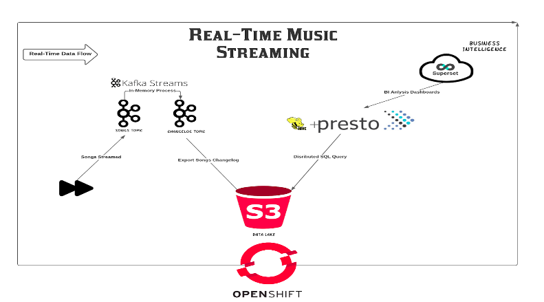
This demo deploys a music streaming application, that generates events based on users’ behavior (will be explained further).
Demo Architecture
Using that data that is being generated, we can use Open Source tools in order to create our dashboards and visualizations, and provide our stakeholders so as our data scientists a more reliable way to visualize important data.
THIS AFFECTS BUSINESS LOGIC DIRECTLY!
Now that the message is clear, let’s start playing!
Prerequisites
A running Ceph Cluster (> RHCS4)
A running Openshift 4 cluster (> 4.6.8)
An OCS cluster, in external mode, to provide both Object and Block storage
Installation
Create a new project in your Openshift cluster, where all resources should be deployed:
$ oc new-project data-engineering-demo
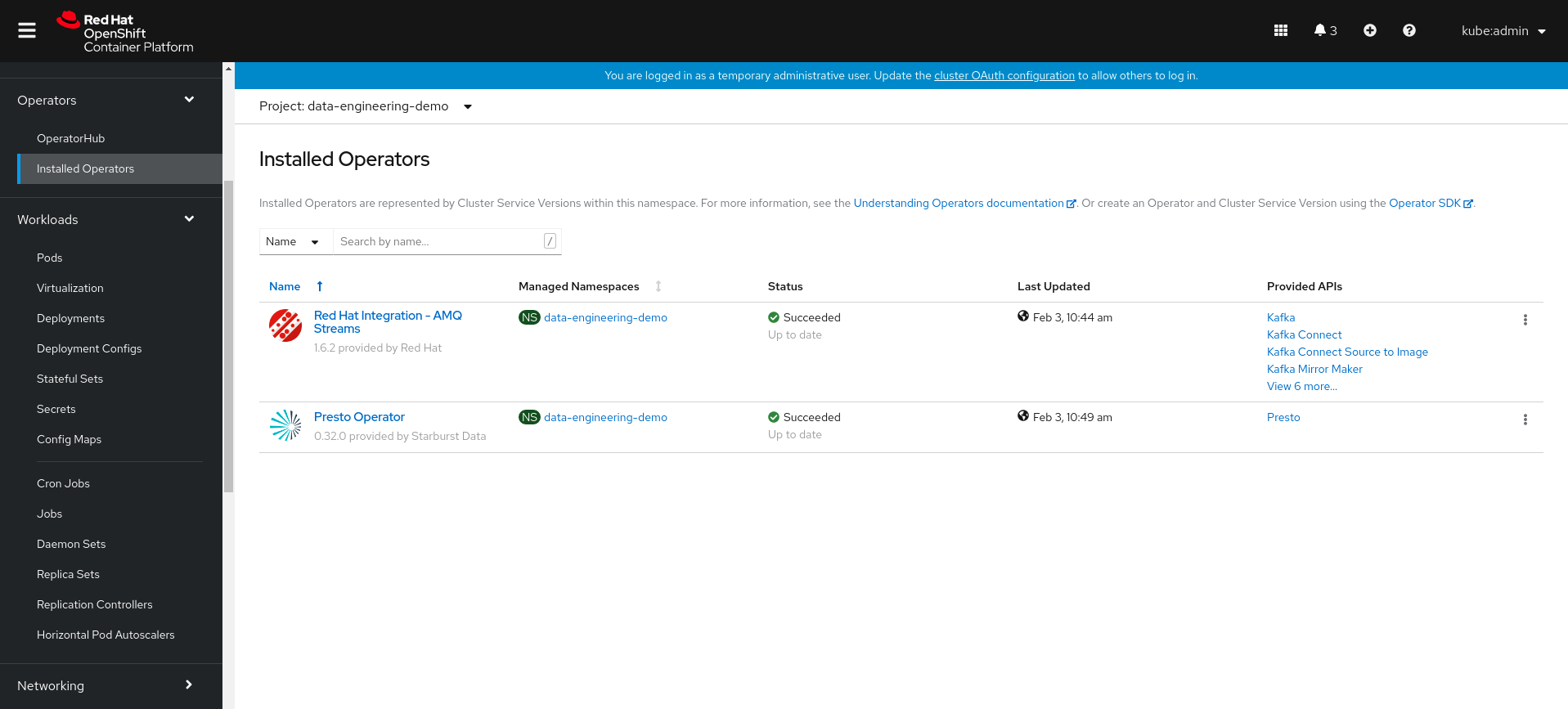
Install both AMQ Streams and Presto Operators, as we’ll need those to create our relevant resources. go the the Operator Hub section on the left panel to install:
Installed Operators in the created project
Clone the needed git repository so you’ll be able to deploy the demo:
Change your directory into the demo directory, where all manifests are located:
$ cd cephdemos/data-engineering-pipeline-demo-ocp
Data Services Preparation
Preparing our S3 environment
Now that we have all the prerequisites ready, let’s start by creating our needed S3 resources. As we are using an external Ceph cluster, we should create the needed S3 user in order to interact with the cluster. Additionally, we need to create an S3 bucket so that Kafka could export our events to the data lake. Let’s create those resources:
The script uses awscli in order to export our credentials as environment variables, so that we’ll be able to create the bucket properly. Make sure that you have access to your endpoint URL with all the open ports so that this script will work properly.
Deploying Kafka new-ETL
Now that we have our S3 ready, we need to deploy all the needed Kafka resources. In this section we’ll deploy a Kafka cluster, using the AMQ Streams operator, that is offered via the Openshift Operator Hub. Additionally, we’ll deploy Kafka Topics and Kafka Connect as well, in order to export all of the existing topic events to our S3 bucket. Important! make sure that you change the endpoint URL to suit yours, or else Kafka Connect will try to expose the events with no success.
Run the script in order to create those resources:
$ cd 02-kafka && ./run.sh && cd ..
Now let’s verify all pods were successfully created:
Those topics will be used by our streaming application to receive, transform and export those events with the proper format, into our S3 bucket. In the end, topic music-chart-songs-store-changelog will hold all the information with its final structure, so that we’ll be able to query it.
Running Presto for Distributed Querying
In this demo, we’ll use Presto’s ability to query S3 bucket prefixes (similar to tables in relational databases). Presto needs a schema to be created, in order to understand what is the file structure that it needs to query, in our example, all events that are being exported to our S3 bucket will look like the following:
{"count":7,"songName":"The Good The Bad And The Ugly"}
Each file will be exported with a JSON structure, that holds two key-value pairs. To emphasize, you can think of it as a table, with two columns where the first one is count and the second is songName, and all files that are being written to the bucket are just rows with this structure.
Now that we have a better understanding of our data structure, we can deploy our Presto cluster. This cluster will create a hive instance to store the schema metadata (with Postgres to store the schema information), and a Presto cluster that contains the coordinator and worker pods. All of those resources will be automatically created by the Presto Operator, which is offered as part of the Openshift Operator Hub as well.
Let’s run the script to create those resources:
$ cd 04-presto && ./run.sh && cd ..
Now let’s verify all pods were successfully created:
$ oc get pods | egrep -e "presto|postgres"
NAME                                                  READY   STATUS    RESTARTS   AGE
hive-metastore-presto-cluster-576b7bb848-7btlw        1/1     Running   0          15s
postgres-68d5445b7c-g9qkj                             1/1     Running   0          77s
presto-coordinator-presto-cluster-8f6cfd6dd-g9p4l     1/2     Running   0          15s
presto-operator-dbbc6b78f-m6p6l                       1/1     Running   0          7h33m
presto-worker-presto-cluster-5b87f7c988-cg9m6         1/1     Running   0          15s
Visualizing real-time data with Superset
Superset is a visualization tool, that can present visualization and dashboards from many JDBC resources, such as Presto, Postgres, etc. As Presto has no real UI that provides us the ability to explore our data, controlling permissions, and RBAC, we’ll use Superset.
Run the script in order to deploy Superset in your cluster:
After we have all of our infrastructure services ready, we need to create the data logic behind our streaming application. As Presto queries data from our S3 bucket, we need to create a schema, that will allow Presto to know how it should query our data, so as a table to provide the structure knowledge.
Change your context to work with the hive catalog:
$ presto-cli --catalog hive
Create a schema, that’ll tell Presto to use the s3a connector in order to query data from our S3 bucket prefix:
$ CREATE SCHEMA hive.songs WITH (location='s3a://music-chart-songs-store-changelog/music-chart-songs-store-changelog.json/');
Change the schema context, and create a table:
$ USE hive.songs;
$ CREATE TABLE songs (count int, songName varchar) WITH (format = 'json', external_location = 's3a://music-chart-songs-store-changelog/music-chart-songs-store-changelog.json/');
Pay attention! creating the table provides Presto the actual knowledge of each file’s structure, as we saw in the previous section. Now let’s try to query our S3 bucket:
We have no data, and it’s OK! we haven’t started streaming any data, but we see that we get no error, which means Presto can access our S3 service.
Streaming Real-Time Events
Now that all resources are ready to use, we can finally deploy our streaming application! Our streaming application is actually a Kafka producer that simulates a media player, it has a pre-defined list of songs that are being randomly “played” by our media player. Each time a user plays a song, the event is being sent to a Kafka topic.
Then, we’re using Kafka Streams, in order to transform the data to our wanted structure. Streams will take each event that is being sent to Kafka, transform it, and write it to another topic, where it’ll be automatically exported to our S3 bucket.
Let’s run the deployment:
$ cd 03-music-chart-app && ./run.sh && cd ..
Let’s verify all pods are running, the player-app pod is our media player, while the music-chart pod is actually a pod that holds all the Kafka Streams logic:
$ oc logs player-app-79fb9cd54f-bhtl52021-02-03 16:28:41,970 INFO  [org.acm.PlaySongsGenerator] (RxComputationThreadPool-1) song 1: The Good The Bad And The Ugly played.
2021-02-03 16:28:46,970 INFO  [org.acm.PlaySongsGenerator] (RxComputationThreadPool-1) song 1: The Good The Bad And The Ugly played.
2021-02-03 16:28:51,970 INFO  [org.acm.PlaySongsGenerator] (RxComputationThreadPool-1) song 2: Believe played.
2021-02-03 16:28:56,970 INFO  [org.acm.PlaySongsGenerator] (RxComputationThreadPool-1) song 3: Still Loving You played.
2021-02-03 16:29:01,972 INFO  [org.acm.PlaySongsGenerator] (RxComputationThreadPool-1) song 2: Believe played.
2021-02-03 16:29:06,970 INFO  [org.acm.PlaySongsGenerator] (RxComputationThreadPool-1) song 7: Fox On The Run played.
We see that we have the data being written randomly, each time a song is being played, an event is being sent to our Kafka topic. Now, let’s take a look at our music-chart logs:
$ oc logs music-chart-576857c7f8-7l65x [KTABLE-TOSTREAM-0000000006]: 2, PlayedSong [count=1, songName=Believe]
[KTABLE-TOSTREAM-0000000006]: 8, PlayedSong [count=1, songName=Perfect]
[KTABLE-TOSTREAM-0000000006]: 3, PlayedSong [count=1, songName=Still Loving You]
[KTABLE-TOSTREAM-0000000006]: 1, PlayedSong [count=1, songName=The Good The Bad And The Ugly]
[KTABLE-TOSTREAM-0000000006]: 6, PlayedSong [count=1, songName=Into The Unknown]
[KTABLE-TOSTREAM-0000000006]: 3, PlayedSong [count=2, songName=Still Loving You]
[KTABLE-TOSTREAM-0000000006]: 5, PlayedSong [count=1, songName=Sometimes]
[KTABLE-TOSTREAM-0000000006]: 2, PlayedSong [count=2, songName=Believe]
[KTABLE-TOSTREAM-0000000006]: 1, PlayedSong [count=2, songName=The Good The Bad And The Ugly]
We see that data is being transformed successfully, and that the count number increases as users play more songs.
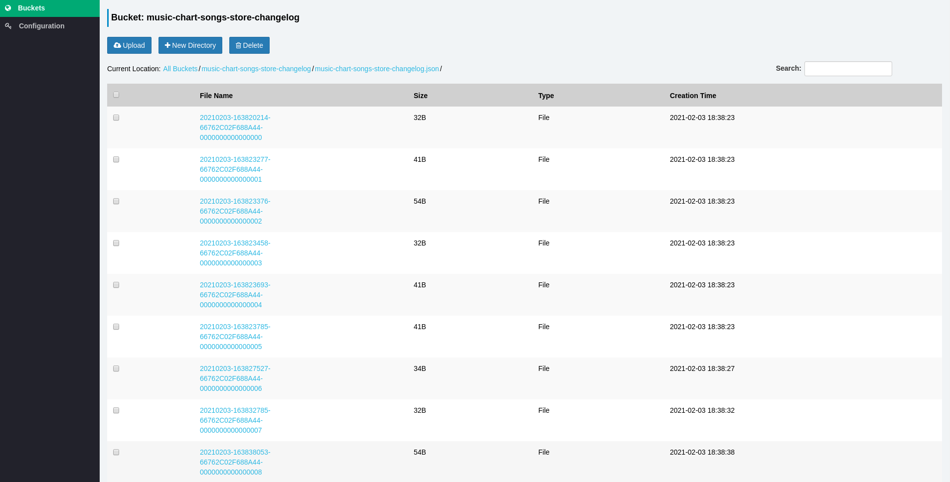
Now, we need to make sure our pipeline works, so let’s go the our S3 service to verify all events are being exported successfully. for this purpose, I’ve used Sree as the S3 browser. Make sure you’re using the right credentials and endpoint URL:
S3 browser of our created bucket prefix
Let’s go back to our Presto coordinator pod and try to query our data again:
$ presto> presto-cli --catalog hive
$ presto:songs> USE hive.songs;
Run the SQL query in order to fetch our data:
$ select * from songs;
 count |           songname
-------+-------------------------------
     1 | Bohemian Rhapsody
     4 | Still Loving You
     1 | The Good The Bad And The Ugly
     3 | Believe
     1 | Perfect
     1 | Sometimes
     2 | The Good The Bad And The Ugly
     2 | Bohemian Rhapsody
     3 | Still Loving You
     4 | Sometimes
     2 | Into The Unknown
     4 | Believe
     4 | Into The Unknown
     2 | Sometimes
     5 | Still Loving You
     3 | The Good The Bad And The Ugly
Amazing! We see that our data is being updated automatically! try running this command a few more times, and you’ll see that the number of rows grows. Now, in order to start visualizing our data, look for the Superset route, where you’ll be able to login to the console:
$ oc get routeNAME       HOST/PORT                                            PATH   SERVICES   PORT       TERMINATION   WILDCARD
superset   superset-data-engineering-demo.apps.ocp.spaz.local          superset   8088-tcp                 None
When we reach our Superset console (login with admin:admin), we can see that we can go to Manage Databases –> Create Database to create our Preto connection, make sure you put your Presto’s ClusterIP service name, at the end make sure you test your connection:
Testing Presto’s connection while creating a database
Now that we can have a more convenient way to query our data, let’s try exploring our data a bit. Go to SQL Lab, and see that you can perform our previous query. To emphasize, watch the following query, that will show how many times each song has been played:
Creating a Query to Visualization
Good! we can query data! feel free to create all your wanted visualizations and dashboards. As an example, I’ve created a dashboard that changes in real-time, as every refresh to the dashboard actually queries all the data from Presto once again:
Real-Time data dashboard
Conclusion
In this demo, we saw how we can leverage Open Source products in order to run automatic data pipelines, all scheduled on Openshift. As Kubernetes breaks the records of adoption, organizations should consider moving their workloads towards Kubernetes, so that their data services won’t be left behind. Using Red Hat and Partner Operators, Openshift offers both day-1 and day-2 management to your data services.
Thank you for reading this blog post, see ya next time 🙂
시계열 데이터는 작업하기가 어렵고 답답할 수 있습니다.아르 자형먹은 모델은 매우 까다 롭고 조정하기 어려울 수 있습니다.이것은특별히여러 계절성이있는 데이터로 작업하는 경우 true입니다.또한 SARIMAX와 같은 기존 시계열 모델에는 정상 성 및 균등 한 간격 값과 같은 엄격한 데이터 요구 사항이 많이 있습니다.장기 기억이있는 반복 신경망 (RNN-LSTM)과 같은 다른 시계열 모델은 신경망 아키텍처에 대한 이해가 부족한 경우 매우 복잡하고 작업하기 어려울 수 있습니다.따라서 평균 데이터 분석가에게는 시계열 분석에 대한 진입 장벽이 높습니다.그래서 2017 년에 페이스 북의 몇몇 연구자들은 오픈 소스 프로젝트를 소개 한“대규모 예측”이라는 논문을 발표했습니다.페이스 북 예언자, 빠르고 강력하며 액세스 가능한 시계열 모델링을 어디서나 데이터 분석가와 데이터 과학자에게 제공합니다.
Facebook Prophet을 더 자세히 살펴보기 위해 먼저 그이면의 수학을 요약 한 다음 Python에서 사용하는 방법을 살펴 보겠습니다 (R에서도 구현할 수 있음).
Facebook Prophet이란 무엇이며 어떻게 작동합니까?
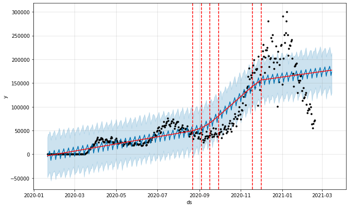
Facebook Prophet은 몇 가지 새로운 변형과 함께 몇 가지 오래된 아이디어를 사용하는 시계열 모델을 생성하기위한 오픈 소스 알고리즘입니다.여러 계절성이 있고 위의 다른 알고리즘의 단점 중 일부에 직면하지 않는 시계열 모델링에 특히 유용합니다.핵심은 세 가지 시간 함수와 오류 항의 합계입니다.g (t), 계절성성), 공휴일h (t)및 오류e_t:
성장 기능 (및 변화 지점) :
성장 함수는 데이터의 전반적인 추세를 모델링합니다.선형 및 로지스틱 함수에 대한 기본 지식이있는 사람에게는 오래된 아이디어가 익숙해야합니다.Facebook 선지자에 통합 된 새로운 아이디어는 성장 추세가 데이터의 모든 지점에 나타나거나 Prophet이 “변경 지점”이라고 부르는 지점에서 변경 될 수 있다는 것입니다.
변경점은 데이터가 방향을 이동하는 데이터의 순간입니다.예를 들어 새로운 COVID-19 사례를 사용하면 백신이 도입 된 후 정점에 도달 한 후 새로운 사례가 떨어지기 시작할 수 있습니다.또는 새로운 균주가 인구에 도입되는 경우 갑작스런 사례가 나타날 수 있습니다.예언자는 변화 지점을 자동으로 감지하거나 직접 설정할 수 있습니다.또한 자동 변경점 감지에서 고려되는 데이터의 양과 성장 기능을 변경하는 데있어 변경점이 갖는 힘을 조정할 수도 있습니다.
성장 기능에는 세 가지 주요 옵션이 있습니다.
선형 성장 :이것은 예언자의 기본 설정입니다.변화 점간에 기울기가 다른 부분 선형 방정식 세트를 사용합니다.선형 성장을 사용하면 성장 기간이 고전과 유사하게 보입니다.y = mx + b중학교부터는 기울기 (m)와 오프셋 (b)은 가변적이며 각 변경점에서 값이 변경됩니다.
물류 성장 :이 설정은 시계열에 모델링하는 값이 포화되고 최대 값 또는 최소값을 초과 할 수없는 상한 또는 하한이있는 경우에 유용합니다 (이동 능력을 고려).물류 성장이 사용되는 경우 성장 기간은 운반 능력 (C)이 시간과 성장률 (k) 및 오프셋의 함수에 따라 달라진다는 점을 제외하고는 물류 곡선 (아래 참조)에 대한 일반적인 방정식과 유사하게 보입니다.(m)은 가변적이며 각 변화 지점에서 값이 변경됩니다.
플랫:마지막으로, 시간이 지남에 따라 성장이 없을 때 플랫 추세를 선택할 수 있습니다 (하지만 여전히 계절성이있을 수 있음).플랫으로 설정하면 성장 기능이 일정한 값이됩니다.
계절성 함수 :
계절성 함수는 단순히 시간 함수로서의 푸리에 급수입니다.푸리에 시리즈에 익숙하지 않은 경우이를 쉽게 생각할 수있는 방법은 연속 된 사인과 코사인의 합입니다.각 사인 및 코사인 항에 일부 계수를 곱합니다.이 합계는 거의 모든 곡선이나 Facebook Prophet의 경우 데이터의 계절성 (주기적 패턴)과 비슷할 수 있습니다.모두 다음과 같이 보입니다.
여전히 푸리에 시리즈를 이해하는 데 어려움을 겪고 있다면 걱정하지 마십시오.Prophet이 시리즈에서 최적의 용어 수 (푸리에 순서라고도 함)를 자동으로 감지하므로 Facebook Prophet을 계속 사용할 수 있습니다.또는 이해에 자신이 있고 더 많은 뉘앙스를 원하는 경우 특정 데이터 세트의 요구 사항에 따라 푸리에 순서를 선택할 수도 있습니다.순서가 높을수록 계열의 용어가 더 많습니다.덧셈과 곱셈 계절성 중에서 선택할 수도 있습니다.
휴일 / 이벤트 기능 :
휴일 기능을 사용하면 Facebook Prophet이 휴일 또는 주요 이벤트로 인해 예측이 변경 될 때 예측을 조정할 수 있습니다.날짜 목록을 사용하고 (미국 공휴일의 기본 제공 날짜가 있거나 사용자가 직접 날짜를 정의 할 수 있음) 예측에 각 날짜가있을 때 과거 데이터를 기반으로 성장 및 계절성 조건에서 예측 값을 더하거나 뺍니다.확인 된 휴일 날짜에.또한 날짜에 따라 다양한 요일을 식별 할 수 있습니다 (크리스마스 / 새해, 휴일 주말, 추수 감사절과 블랙 프라이데이 / 사이버 먼데이 등).
Facebook Prophet 사용 및 조정 방법
R 또는 Python으로 구현할 수 있지만이 블로그에서는 Python에서의 사용에 중점을 둘 것입니다.Python 3.7 이상이 필요합니다.설치하기 위해서:
$ pip install pystan
$ pip 설치 fbprophet
Prepare the data
pandas를 사용하여 데이터를 읽고 정리 한 후에는 거의 Facebook Prophet을 사용할 준비가되었습니다.그러나 Facebook Prophet에서는 시계열의 날짜가 제목의 열에 있어야합니다.ds및 제목 열의 시리즈 값와이.물류 성장을 사용하는 경우 추가로 추가해야합니다.캡과바닥시계열의 각 특정 시간 항목에서 가능한 증가의 최대 값 및 최소값이있는 열.
데모를 위해 New York Times가 Github에서 추적 한 새로운 COVID-19 사례를 사용합니다.먼저 위의 형식으로 데이터를 읽고 준비합니다.여기에 물류 성장이있는 것 같지 않기 때문에ds과와이열 :
기본 Facebook Prophet 모델 실행
Facebook Prophet은 scikit-learn과 유사하게 작동하므로 먼저 모델을 인스턴스화 한 다음.fit (ts)그것을 통해 시계열을 전달합니다.전화 할 때.predict (ts), 예언자는 많은 정보를 출력합니다.운 좋게도 개발자는.make_future_dataframe (기간 = 10)모든 출력물을 체계적으로 쉽게 수집 할 수 있습니다.이 메서드는 다음을 사용하여 예측으로 채울 빈 Pandas 데이터 프레임을 출력합니다..predict (ts)방법.예측에는 데이터 세트에있는 모든 과거 값에 대한 예측과 메서드를 통해 전달 된 기간 수에 대한 추가 예측이 포함됩니다 (10을 초과하는 경우).이 미래 데이터 프레임에는 유용한 정보 열이 많이 있지만 가장 중요한 열은 다음과 같습니다.
ds예측의 타임 스탬프 항목을 포함합니다.
야트시계열의 예측 값을 포함합니다.
yhat_lower예측에 대한 신뢰 구간의 하단을 포함합니다.
yhat_upper예측에 대한 신뢰 구간의 하단을 포함합니다.
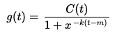
ㅏ.음모()또한 원래 데이터, 예측 및 모델의 신뢰 구간을 쉽게 플로팅 할 수 있도록 기능이 제공됩니다.이 모델의 첫 번째 반복에서는 Prophet이 자동으로 하이퍼 파라미터를 선택하도록 할 것입니다.
그러면 다음과 같은 플롯 된 예측이 출력됩니다.
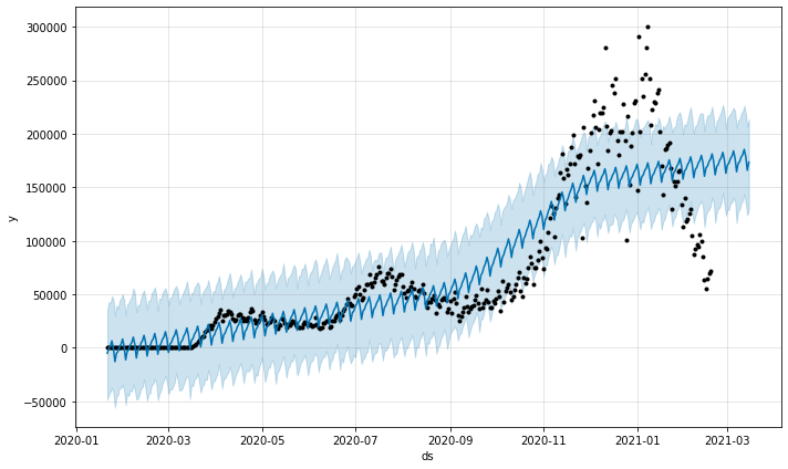
다음 코드를 추가하여 위의 플롯에 변경점을 추가 할 수도 있습니다.
하이퍼 파라미터를 조정하지 않은 것을 고려하면 꽤 괜찮은 것 같습니다!예언자는 새로보고 된 사례의 주간 계절 성과 (아마도 테스트 장소의 주말 시간이 다르기 때문에) 전체적인 상승 추세를 확인했습니다.또한 새로운 사례의 비율이 크게 증가하는 것을 더 잘 모델링하기 위해 여름과 가을에 변화 지점을 추가했습니다.그러나 시각적으로 전반적으로 훌륭한 모델처럼 보이지 않으며 원본 데이터의 많은 주요 추세를 놓치고 있습니다.따라서 무슨 일이 일어나고 있는지 더 잘 평가하기 위해 조정해야합니다.
Facebook Prophet 조정
위 모델의 주요 문제 중 일부를 수정 해 보겠습니다.
침체를 놓친다 :예언자는 새해 이후 새로운 COVID 사례에 침체를 통합 할 수 없었습니다.이는 변경점을 식별 할 때 고려되는 데이터 포인트 범위의 기본 설정이 시계열 데이터의 처음 80 %이기 때문입니다.이 문제는changepoint_range = 1데이터의 100 %를 통합 할 모델을 인스턴스화 할 때.다른 상황에서는 모델이 데이터에 과적 합하지 않고 마지막 20 %를 스스로 이해할 수 있도록 변경점 범위를 80 % 이하로 유지하는 것이 좋습니다.하지만이 경우 지금까지 발생한 상황을 정확하게 모델링하려고하기 때문에 조정을 100 %로 허용합니다.
변화 지점의 강점 :위대한 선지자는 변화 지점을 만들 수 있었지만 시각적으로 일부 변화 지점이 모델에 미치는 영향이 매우 약하거나 변화 지점이 충분하지 않은 것처럼 보입니다.그만큼changepoint_prior_scale그리고n_changepoints하이퍼 파라미터를 사용하면이를 조정할 수 있습니다.기본적으로,changepoint_prior_scale이 값을 늘리면 더 많은 변경점을 자동으로 감지 할 수 있고 감소하면 더 적게 허용합니다.또는 다음을 사용하여 감지 할 여러 변경점을 지정할 수 있습니다.n_changepoints또는 직접 사용하여 변경점을 나열하십시오.변경점.변경점이 너무 많으면 과적 합이 발생할 수 있으므로주의하십시오.
계절성으로 인한 과적 합 가능성 :새로운 사례의 주간 계절성을 파악한 것은 멋지지만,이 특정 상황에서는 유행병이 언제 끝날지 예측하기 위해 사례의 전반적인 추세를 이해하는 것이 더 중요합니다.Prophet에는 매일, 매주 및 매년 계절성을 조정할 수있는 하이퍼 파라미터가 내장되어 있습니다.그래서 우리는weekly_seasonality = False.또는 사용자 지정 계절성을 만들고 다음을 사용하여 푸리에 순서를 조정할 수 있습니다..add_seasonality ()방법을 사용하거나 다음을 사용하여 자동 계절성을 완화 할 수 있습니다.season_prior_scale하이퍼 파라미터.그러나이 경우 이러한 옵션 중 하나를 사용하는 것은 약간 과잉 일 수 있습니다.
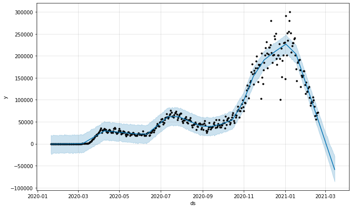
이러한 변경 사항으로 모델을 다시 실행하면 다음이 생성됩니다.
와!하이퍼 파라미터에 대한 세 가지 작은 변경을 통해 지난 1 년 동안 새로운 COVID 사례의 행동에 대한 매우 정확한 모델을 확보했습니다.이 모델에서는 3 월 초에 사례가 거의 0에 가까워 질 것으로 예측합니다.케이스가 점근 적으로 감소하기 때문에 이것은 아마도 가능성이 낮습니다.
Facebook Prophet은 사용하기 쉽고 빠르며 다른 종류의 시계열 모델링 알고리즘이 직면하는 많은 문제에 직면하지 않습니다 (제가 가장 좋아하는 것은 결 측값을 가질 수 있다는 것입니다!).API에는 다음이 포함됩니다.선적 서류 비치앞으로 나아가고 교차 검증을 사용하고 외부 변수를 통합하는 방법 등에 대해 설명합니다.당신은 또한 확인할 수 있습니다이 GitHub 저장소이 블로그에 사용 된 코드가 포함 된 Jupyter 노트북 용입니다.
Time series data can be difficult and frustrating to work with, and the various algorithms that generate models can be quite finicky and difficult to tune. This is particularly true if you are working with data that has multiple seasonalities. In addition, traditional time series models like SARIMAX have many stringent data requirements like stationarity and equally spaced values. Other time series models like Recurring Neural Networks with Long-Short Term Memory (RNN-LSTM) can be highly complex and difficult to work with if you don’t have a significant level of understanding about neural network architecture. So for the average data analyst, there is a high barrier of entry to time series analysis. So in 2017, a few researchers at Facebook published a paper called, “Forecasting at Scale” which introduced the open-source project Facebook Prophet, giving quick, powerful, and accessible time-series modeling to data analysts and data scientists everywhere.
To further explore Facebook Prophet, I’m going to first summarize the math behind it and then go over how to use it in Python (although it can also be implemented in R).
What is Facebook Prophet and how does it work?
Facebook Prophet is an open-source algorithm for generating time-series models that uses a few old ideas with some new twists. It is particularly good at modeling time series that have multiple seasonalities and doesn’t face some of the above drawbacks of other algorithms. At its core is the sum of three functions of time plus an error term: growthg(t), seasonality s(t), holidays h(t) , and error e_t :
The Growth Function (and change points):
The growth function models the overall trend of the data. The old ideas are should be familiar to anyone with a basic knowledge of linear and logistic functions. The new idea incorporated into Facebook prophet is that the growth trend can be present at all points in the data or can be altered at what Prophet calls “changepoints”.
Changepoints are moments in the data where the data shifts direction. Using new COVID-19 cases as an example, it could be due to new cases beginning to fall after hitting a peak once a vaccine is introduced. Or it could be a sudden pick up of cases when a new strain is introduced into the population and so on. Prophet can automatically detect change points or you can set them yourself. You can also adjust the power the change points have in altering the growth function and the amount of data taken into account in automatic changepoint detection.
The growth function has are three main options:
Linear Growth: This is the default setting for Prophet. It uses a set of piecewise linear equations with differing slopes between change points. When linear growth is used, the growth term will look similar to the classic y = mx + b from middle school, except the slope(m) and offset(b) are variable and will change value at each changepoint.
Logistic Growth: This setting is useful when your time series has a cap or a floor in which the values you are modeling becomes saturated and can’t surpass a maximum or minimum value (think carrying capacity). When logistic growth is used, the growth term will look similar to a typical equation for a logistic curve (see below), except it the carrying capacity (C) will vary as a function of time and the growth rate (k) and the offset(m) are variable and will change value at each change point.
Flat: Lastly, you can choose a flat trend when there is no growth over time (but there still may be seasonality). If set to flat the growth function will be a constant value.
The Seasonality Function:
The seasonality function is simply a Fourier Series as a function of time. If you are unfamiliar with Fourier Series, an easy way to think about it is the sum of many successive sines and cosines. Each sine and cosine term is multiplied by some coefficient. This sum can approximate nearly any curve or in the case of Facebook Prophet, the seasonality (cyclical pattern) in our data. All together it looks like this:
If you are still struggling to understand the Fourier series, do not worry. You can still use Facebook Prophet because Prophet will automatically detect an optimal number of terms in the series, also known as the Fourier order. Or if you are confident in your understanding and want more nuance, you can also choose the Fourier order based on the needs of your particular data set. The higher the order the more terms in the series. You can also choose between additive and multiplicative seasonality.
The Holiday/Event Function:
The holiday function allows Facebook Prophet to adjust forecasting when a holiday or major event may change the forecast. It takes a list of dates (there are built-in dates of US holidays or you can define your own dates) and when each date is present in the forecast adds or subtracts value from the forecast from the growth and seasonality terms based on historical data on the identified holiday dates. You can also identify a range of days around dates (think the time between Christmas/New Years, holiday weekends, thanksgiving’s association with Black Friday/Cyber Monday, etc).
How to use and tune Facebook Prophet
It can be implemented in R or Python, but we’ll focus on use in Python in this blog. You’ll need at least Python 3.7. To install:
$pip install pystan
$pip install fbprophet
Prepare the data
After reading in data and cleaning using pandas, you are almost ready to use Facebook Prophet. However, Facebook Prophet requires that the dates of your time series are located in a column titled ds and the values of the series in a column titled y. Note that if you are using logistic growth you’ll also need to add additional cap and floor columns with the maximum and minimum values of the possible growth at each specific time entry in the time series.
For demonstration, we’ll use new COVID-19 cases tracked by the New York Times on Github. First, we read and prepare the data in the form above. It doesn’t seem like there is logistic growth here so we’ll just focus on creating the ds and y columns:
Run a basic Facebook Prophet model
Facebook Prophet operates similarly to scikit-learn, so first we instantiate the model, then call .fit(ts) passing the time series through it. When calling .predict(ts), Prophet outputs a lot of information. Luckily, the developers added a method called .make_future_dataframe(periods = 10) that will easily collect all of the output in an organized way. This method outputs an empty pandas dataframe that we will fill with the forecast using the .predict(ts)method. The forecast will contain a prediction for every historical value present in the dataset plus additional forecasts for the number of periods passed through the method (in the case above 10). There are many columns of useful information in this future dataframe but the most important ones are:
ds contains the timestamp entry of the forecast
yhat contains the forecasted value of the time series
yhat_lower contains the bottom of the confidence interval for the forecast
yhat_upper contains the bottom of the confidence interval for the forecast
A .plot() function is also provided for easy plotting of the original data, the forecast and the confidence interval of the model. In this first iteration of the model we will allow Prophet to automatically choose the hyperparameters:
This outputs the following plotted forecast:
You can also add changepoints to the above plot by adding the following code:
Seems pretty decent, considering we didn’t tune any hyperparameters! Prophet picked up on a weekly seasonality of newly reported cases (probably due to differing weekend hours of testing sites) and an overall upward trend. It also added change points when during the summer and fall to better model the large increase in the rate of new cases. However, it doesn’t visually seem like a great model overall and misses many key trends in the original data. So we’ll need to tune it to get a better assessment of what is going on.
Tuning Facebook Prophet
Let’s fix some of the key problems our above model has:
Misses the downturn: Prophet was unable to incorporate the downturn in new COVID cases after the new year. This is because the default setting for the range of data points considered when identifying changepoints is the first 80% of data in the time series. We can fix this by setting changepoint_range = 1 when instantiating the model which will incorporate 100% of the data. In other situations, it may be good to keep the changepoint range at 80% or lower to ensure that the model doesn’t overfit your data and can understand the last 20% on its own. But, in this case, because we are just trying to accurately model what has happened so far, we’ll allow the adjustment to 100%.
Strength of changepoints: While its great prophet was able to create change points, it visually seems like some of the changepoints are quite weak in impact on the model, or possibly there aren’t enough changepoints. The changepoint_prior_scale and the n_changepoints hyperparameters allow us to adjust this. By default, changepoint_prior_scale it is set to 0.05, increasing this value allows the automatic detection of more change points and decreases it allows for less. Alternatively, we can specify a number of changepoints to detect using n_changepoints or list the changepoints ourselves using changepoints. Be careful with this, as too many changepoints may cause overfitting.
Possible overfitting due to seasonality: While it’s cool that it picked up on the weekly seasonality of new cases, in this particular context it’s more important to understand the overall trend of cases to possibly predict when the pandemic will end. Prophet has built-in hyperparameters to allow you to adjust daily, weekly and yearly seasonality. So we can fix this by setting weekly_seasonality = False. Alternatively, we could try to create our own custom seasonality and adjust the Fourier order using the.add_seasonality()method or we could dampen the automatic seasonality using the seasonality_prior_scale hyperparameter. However, in this case, it might be a little overkill to use either of those options
Running the model again with these changes yields:
Wow! With three small changes to the hyperparameters, we have a pretty accurate model of the behavior of new COVID cases over the past year. In this model, it predicts that cases will be near zero in early March. This is probably unlikely, as cases will probably decrease asymptotically.
Facebook Prophet is easy to use, fast, and doesn’t face many of the challenges that some other kinds of time-series modeling algorithms face (my favorite is that you can have missing values!). The API also includes documentation on how to use walk forward and cross validation, incorporate exogenous variables, and more. You can also check out this GitHub repository for the Jupyter Notebooks containing the code used in this blog.