None
DataAnalytics(en)
Deep Learning with Keras Cheat Sheet (2021), Python for Data Science
Deep Learning with Keras Cheat Sheet (2021), Python for Data Science
The absolute basics for beginners learning Keras for Deep Learning in 2021

Keras is a powerful and easy-to-use deep learning library for TensorFlow that provides high-level neural network APIs to develop and evaluate deep learning models.
Check out the sections below to learn how to optimize Keras to create various deep learning models.
Sections:
1. Basic Example
2. Data
3. Preprocessing
4. Model Architecture
5. Compile Model
6. Model Training
7. Prediction
8. Evaluate Your Models’ Performance
9. Save/Reload Models
Basic Example
The code below demonstrates the basic steps of using Keras to create and run a deep learning model on a set of data.
The steps in the code include: loading the data, preprocessing the data, creating the model, adding layers to the model, fitting the model on the data, using the trained model to make predictions on the test set, and finally evaluating the performance of the model.
>>> import numpy as np
>>> from keras.models import Sequential
>>> from keras.layers import Dense
>>> from keras.datasets import boston_housing
>>> (x_train, y_train),(x_test, y_test) = boston_housing.load_data()
>>> model = Sequential()
>>> model.add(Dense(12,activation='relu',input_dim= 8))
>>> model.add(Dense(1))
>>> model.compile(optimizer='rmsprop',loss='mse',metrics=['mae']))
>>> model.fit(x_train,y_train,batch_size=32,epochs=15)
>>> model.predict(x_test, batch_size=32)
>>> score = model.evaluate(x_test,y_test,batch_size=32)
Data
Your data needs to be stored as NumPy arrays or as a list of NumPy arrays. Ideally, you split the data in training and test sets, for which you can also resort to the train_test_split module of sklearn.cross_validation.
For an example dataset, you can use the Boson Housing dataset that is incorporated in the Keras library.
>>> from keras.datasets import boston_housing
>>> (x_train, y_train),(x_test, y_test) = boston_housing.load_data()
Preprocessing
After a dataset is imported it may not be ready for a model to be fit onto it. In this case, you have to do some preprocessing to prepare the data for the model.
Encoding Categorical Features
Encode’s target labels with values between 0 and n_classes-1.
>>> from keras.utils import to_categorical
>>> Y_train = to_categorical(y_train, num_classes)
>>> Y_test = to_categorical(y_test, num_classes)
Train and Test Sets
Splits the dataset into training and test sets for both the X and y variables.
>>> from sklearn.model_selection import train_test_split
>>> X_train,X_test,y_train,y_test = train_test_split(X, y,
    test_size=0.33,random_state=42)
Standardization
Standardize’s the features by removing the mean and scaling to unit variance.
>>> from sklearn.preprocessing import StandardScaler
>>> scaler = StandardScaler().fit(x_train)
>>> standardized_X = scaler.transform(x_train)
>>> standardized_X_test = scaler.transform(x_test)
Model Architecture
In this section, you’ll learn how to build different deep learning models layer by layer.
Sequential Model
A Sequential model is appropriate for a plain stack of layers where each layer has exactly one input tensor and one output tensor. This is typically the first layer you would add in any model.
>>> from keras.models import Sequential
>>> model = Sequential()
Artificial Neural Network (ANN)
Deep learning model used for classification and regression.
Binary Classification:
The code below is an example of an ANN model used for binary classification (identifying a class as 0 or 1). The code adds 3 layers to the model. The first is the input layer and has 12 nodes, the second layer has 8 nodes, and the last layer has 1 which is the output node or what is predicted.
>>> from keras.layers import Dense
>>> model.add(Dense(12,input_dim=8,kernel_initializer='uniform',
    activation='relu'))
>>> model.add(Dense(8,kernel_initializer='uniform',activation='relu'))
>>> model.add(Dense(1,kernel_initializer='uniform',activation='sigmoid'))
Multi-Class Classification:
The code below is an example of an ANN model used for multi-class classification. The code adds 4 layers to the model. The first is the input layer and has 52 nodes, the second is a dropout layer used to reduce overfitting, the third layer has 52 nodes, and the last layer has 10 nodes which are the probabilities that a certain observation goes into one of 10 different classes.
>>> from keras.layers import Dropout
>>> model.add(Dense(52,activation='relu'),input_shape=(78,))
>>> model.add(Dropout(0.2))
>>> model.add(Dense(52,activation='relu'))
>>> model.add(Dense(10,activation='softmax'))
Regression:
The code below is an example of an ANN model used for regression. The code adds 2 layers to the model. The first is the input layer which has 64 nodes, and the second is the output layer having just 1 node which is the value predicted.
>>> model.add(Dense(64,activation='relu',input_dim=train_data.shape[1]))
>>>
model.add(Dense(1))
Convolution Neural Network (CNN)
Deep learning model used for the classification of pictures. The model is fairly complicated and includes quite a bit of layers which you can see in the code below. That code gives a basic example of what a CNN model looks like.
If you want to have an understanding of what each layer does check out the explanations in the Keras documentation.
>>> from keras.layers import Activation,Conv2D,MaxPooling2D,Flatten >>> model2.add(Conv2D(32,(3,3),padding='same',input_shape=x_train.shape[1:]))
>>> model2.add(Activation('relu'))
>>> model2.add(Conv2D(32,(3,3)))
>>> model2.add(Activation('relu'))
>>> model2.add(MaxPooling2D(pool_size=(2,2)))
>>> model2.add(Dropout(0.25))
>>> model2.add(Conv2D(64,(3,3), padding='same'))
>>> model2.add(Activation('relu'))
>>> model2.add(Conv2D(64,(3, 3)))
>>> model2.add(Activation('relu'))
>>> model2.add(MaxPooling2D(pool_size=(2,2)))
>>> model2.add(Dropout(0.25))
>>> model2.add(Flatten())
>>> model2.add(Dense(512))
>>> model2.add(Activation('relu'))
>>> model2.add(Dropout(0.5))
>>> model2.add(Dense(num_classes))
>>> model2.add(Activation('softmax'))
Recurrent Neural Network (RNN)
Deep learning model used for the time series.
The code below is an example of an RNN model used for time series. The code adds 3 layers to the model. The first layer is the input layer, the second layer is something called Long Short Term Memory, and the third layer is the output layer or what’s predicted from the model.
>>> from keras.klayers import Embedding,LSTM
>>> model.add(Embedding(20000,128))
>>> model.add(LSTM(128,dropout=0.2,recurrent_dropout=0.2))
>>> model.add(Dense(1,activation='sigmoid'))
Compile Model
After a model is constructed you would then compile the model. Compiling just refers to specifying what training configurations (optimizer, loss, metrics) are going to be used to train and evaluate the model.
ANN: Binary Classification
Use these training configurations for an ANN model used for binary classification.
>>> model.compile(optimizer='adam',
                  loss='binary_crossentropy',
                  metrics=['accuracy'])
ANN: Multi-Class Classification
Use these training configurations for an ANN model used for multi-class classification.
>>> model.compile(optimizer='rmsprop',
                  loss='categorical_crossentropy',
                  metrics=['accuracy'])
ANN: Regression
Use these training configurations for an ANN model used for regression.
>>> model.compile(optimizer='rmsprop',
                  loss='mse',
                  metrics=['mae'])
Recurrent Neural Network
Use these training configurations for an RNN model.
>>> model.compile(loss='binary_crossentropy',
                  optimizer='adam',
                  metrics=['accuracy'])
Model Training
After compiling the model, you would now fit it onto your training set. Batch size determines how many observations are inputted into the model at one time, and epochs represent the number of times you want the model to be fit on the training set.
>>> model.fit(x_train,
              y_train,
              batch_size=32,
              epochs=15)
Prediction
Predicting the test set using the trained model
>>> model.predict(x_test, batch_size=32)
Evaluate Your Model’s Performace
Determine how well the model performed on the test set.
>>> score = model.evaluate(x_test,y_test,batch_size=32)
Save/Reload Models
Deep learning models can take quite a long time to train and run, so when they are finished you can save and load them again so you don’t have to go through that process.
>>> from keras.models import load_model
>>> model.save('model_file.h5')
>>> my_model = load_model('my_model.h5')
Python is the top dog when it comes to data science for now and in the foreseeable future. Knowledge of Keras, one of its most powerful libraries for Deep Learning, is often a requirement for Data Scientists today.
Use this cheat sheet as a guide in the beginning and come back to it when needed, and you’ll be well on your way to mastering the Keras library.
If you want to learn more about the Keras library and functions I didn’t cover check out the documentation for Keras, as there are still plenty of useful functions you should learn.
There is more to ‘pandas.read_csv()’ than meets the eye
Tips and Tricks
There is more to ‘pandas.read_csv()’ than meets the eye
A deep dive into some of the parameters of the read_csv function in pandas

Pandas is one of the most widely used libraries in the Data Science ecosystem. This versatile library gives us tools to read, explore and manipulate data in Python. The primary tool used for data import in pandas is read_csv().This function accepts the file path of a comma-separated value, a.k.a, CSV file as input, and directly returns a panda’s dataframe. A comma-separated values (CSV) file is a delimited text file that uses a comma to separate values.
The pandas.read_csv()has about 50 optional calling parameters permitting very fine-tuned data import. This article will touch upon some of the lesser-known parameters and their usage in data analysis tasks.
pandas.read_csv() parameters
The syntax for importing a CSV file in pandas using default parameters is as follows:
import pandas as pd
df = pd.read_csv(filepath)
1. verbose
The verbose parameter, when set to True prints additional information on reading a CSV file like time taken for:
- type conversion,
- memory cleanup, and
- tokenization.
import pandas as pd
df = pd.read_csv('fruits.csv',verbose=True)

2. Prefix
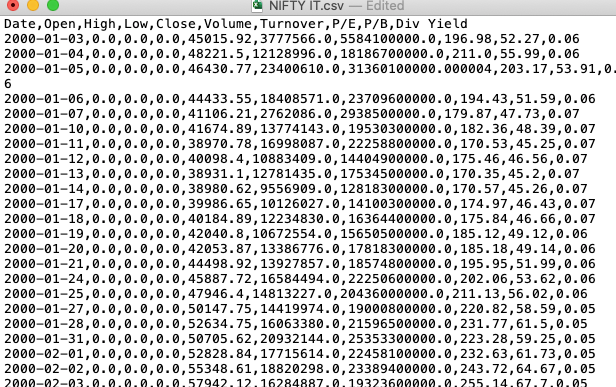
The header is a row in a CSV file containing information about the contents in every column. As the name suggests, it appears at the top of the file.
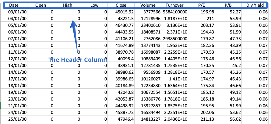
Sometimes a dataset doesn’t contain a header. To read such files, we have to set the header parameter to none explicitly; else, the first row will be considered the header.
df = pd.read_csv('fruits.csv',header=none)
df

The resulting dataframe consists of column numbers in place of column names, starting from zero. Alternatively, we can use the prefix parameter to generate a prefix to be added to the column numbers.
df = pd.read_csv('fruits.csv',header=None, prefix = 'Column')
df
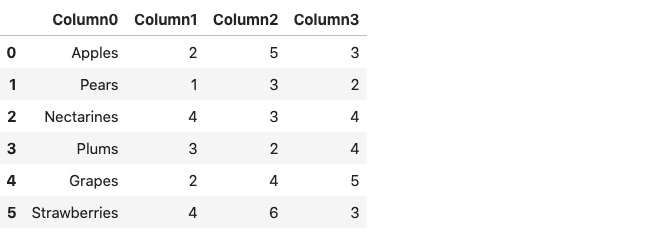
Note that instead of Column, you can specify any name of your choice.
3. mangle_dupe_cols
If a dataframe consists of duplicate column names — ‘X’,’ X’ etcmangle_dupe_cols automatically changes the name to ‘X’, ‘X1’ and differentiate between the repeated columns.
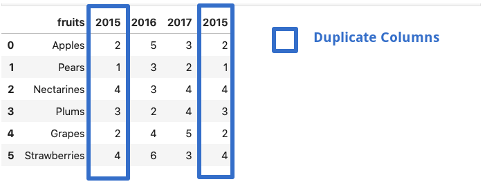
df = pd.read_csv('file.csv',mangle_dupe_cols=True)
df
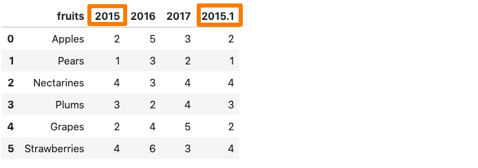
One of the 2015 column in the dataframe get renames as 2015.1.
4. chunksize
The pandas.read_csv() function comes with a chunksize parameter that controls the size of the chunk. It is helpful in loading out of memory datasets in pandas. To enable chunking, we need to declare the size of the chunk in the beginning. This returns an object we can iterate over.
chunk_size=5000
batch_no=1
for chunk in pd.read_csv('yellow_tripdata_2016-02.csv',chunksize=chunk_size):
    chunk.to_csv('chunk'+str(batch_no)+'.csv',index=False)
    batch_no+=1
In the example above, we choose a chunk size of 5000, which means at a time, only 5000 rows of data will be imported. We obtain multiple chunks of 5000 rows of data each, and each chunk can easily be loaded as a pandas dataframe.
df1 = pd.read_csv('chunk1.csv')
df1.head()
You can read more about chunking in the article mentioned below:
5. compression
A lot of times, we receive compressed files. Well, pandas.read_csv can handle these compressed files easily without the need to uncompress them. The compression parameter by default is set to infer, which can automatically infer the kind of files i.e gzip , zip , bz2 , xz from the file extension.
df = pd.read_csv('sample.zip') or the long form:df = pd.read_csv('sample.zip', compression='zip')
6. thousands
Whenever a column in the dataset contains a thousand separator, pandas.read_csv() reads it as a string rather than an integer. For instance, consider the dataset below where the sales column contains a comma separator.
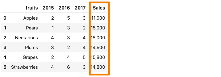
Now, if we were to read the above dataset into a pandas dataframe, the Sales column would be considered as a string due to the comma.
df = pd.read_csv('sample.csv')
df.dtypes

To avoid this, we need to explicitly tell the pandas.read_csv() function that comma is a thousand place indicator with the help of the thousands parameter.
df = pd.read_csv('sample.csv',thousands=',')
df.dtypes

7. skip_blank_lines
If blank lines are present in a dataset, they are automatically skipped. If you want the blank lines to be interpreted as NaN, set the skip_blank_lines option to False.
8. Reading multiple CSV files
This is not a parameter but just a helpful tip. To read multiple files using pandas, we generally need separate data frames. For example, in the example below, we call the pd.read_csv() function twice to read two separate files into two distinct data frames.
df1 = pd.read_csv('dataset1.csv')
df2 = pd.read_csv('dataset2.csv')
One way of reading these multiple files together would be by using a loop. We’ll create a list of the file paths and then iterate through the list using a list comprehension, as follows:
filenames = ['dataset1.csv', 'dataset2,csv']
dataframes = [pd.read_csv(f) for f in filenames]
When many file names have a similar pattern, the glob module from the Python standard library comes in handy. We first need to import the glob function from the built-in glob module. We use the pattern NIFTY*.csv to match any strings that start with the prefix NIFTY and end with the suffix .CSV. The ‘*’(asterisk) is a wild card character. It represents any number of standard characters, including zero.
import glob
filenames = glob.glob('NIFTY*.csv')
filenames
--------------------------------------------------------------------
['NIFTY PHARMA.csv',
 'NIFTY IT.csv',
 'NIFTY BANK.csv',
 'NIFTY_data_2020.csv',
 'NIFTY FMCG.csv']
The code above makes it possible to select all CSV filenames beginning with NIFTY. Now, they all can be read at once using the list comprehension or a loop.
dataframes = [pd.read_csv(f) for f in filenames]
Conclusion
In this article, we looked at a few parameters of the pandas.read_csv() function. it is a beneficial function and comes with a lot of inbuilt parameters which we seldom use. One of the primary reasons for not doing so is because we rarely care to read the documentation. It is a great idea to explore the documentation in detail to unearth the vital information that it may contain.
Data Engineers of Netflix — Interview with Samuel Setegne
Data Engineers of Netflix — Interview with Samuel Setegne
This post is part of our “Data Engineers of Netflix” interview series, where our very own data engineers talk about their journeys to Data Engineering @ Netflix.
Samuel Setegne is a Senior Software Engineer on the Core Data Science and Engineering team. Samuel and his team build tools and frameworks that support data engineering teams across Netflix. In this post, Samuel talks about his journey from being a clinical researcher to supporting data engineering teams.
Samuel comes from West Philadelphia, and he received his Master’s in Biotechnology from Temple University. Before Netflix, Samuel worked at Travelers Insurance in the Data Science & Engineering space, implementing real-time machine learning models to predict severity and complexity at the onset of property claims.
His favorite TV shows: Bojack Horseman, Marco Polo, and The Witcher
His favorite movies: Scarface, I Am Legend and The Old Guard
Sam, what drew you to data engineering?
Early in my career, I was headed full speed towards life as a clinical researcher. Many healthcare practitioners had strong hunches and wild theories that were exciting to test against an empirical study. I personally loved looking at raw data and using it to understand patterns in the world through technology. However, most challenges that came with my role were domain-related but not as technically demanding. For example — clinical data was often small enough to fit into memory on an average computer and only in rare cases would its computation require any technical ingenuity or massive computing power. There was not enough scope to explore the distributed and large-scale computing challenges that usually come with big data processing. Furthermore, engineering velocity was often sacrificed owing to rigid processes.
Moving into pure Data engineering not only offered me the technical challenges I’ve always craved for but also the opportunity to connect the dots through data which was the best of both worlds.
What is your favorite project or a project you’re particularly proud of?
The very first project I had the opportunity to work on as a Netflix contractor was migrating all of Data Science and Engineering’s Python 2 code to Python 3. This was without a doubt, my favorite project that also opened the door for me to join the organization as a full-time employee. It was thrilling to analyze code from various cross-functional teams and learn different coding patterns and styles.
This kind of exposure opened up opportunities for me to engage with various data engineering teams and advocate for python best practices that helped me drive greater impact at Netflix.
What drew you to Netflix?
What initially caught my attention about a chance to work at Netflix was the variety and quality of content. My family and friends were always ecstatic about having lively and raucous conversations about Netflix shows or movies they recently watched like Marco Polo and Tiger King.
Although other great companies play a role in our daily lives, many of them serve as a kind of utility, whereas Netflix is meant to make us live, laugh, and love by enabling us to experience new voices, cultures, and perspectives.
After I read Netflix’s culture memo, I was completely sold. It precisely described what I always knew was missing in places I’ve worked before. I found the mantra of “people over process” extremely refreshing and eventually learned that it unlocked a bold and creative part of me in my technical designs. For instance, if I feel that a design of an application or a pipeline would benefit from new technology or architecture, I have the freedom to explore and innovate without excessive red tape. Typically in large corporations, you’re tied to strict and redundant processes, causing a lot of fatigue for engineers. When I landed at Netflix, it was a breath of fresh air to learn that we lean into freedom and responsibility and allow engineers to push the boundaries.
Sam, how do you approach building tools/frameworks that can be used across data engineering teams?
My team provides generalized solutions for common and repetitive data engineering tasks. This helps provide “paved path” solutions for data engineering teams and reduces the burden of re-inventing the wheel. When you have many specialized teams composed of highly skilled engineers, the last thing you want for a data engineer is to spend too much time solving small problems that are usually buried inside of the big, broad, and impactful problems. When we extrapolate that to every engineer on every Data Science & Engineering team, it easily adds up and is something worth optimizing.
Any time you have a data engineer spending cycles working on tasks where the data engineering part of their brain is turned off, that’s an opportunity where better tooling can help.
For example, many data engineering teams have to orchestrate notification campaigns when they make changes to critical tables that have downstream dependencies. This is achievable by a Data Engineer but it can be very time-consuming, especially having to track the migration of these downstream users over to your new table or table schema to ensure it’s safe to finalize your changes. This problem was tackled by one of my highly skilled team members who built a centralized migration service that lets Data Engineers easily start “migration campaigns” that can automatically identify downstream users and provide notification and status-tracking capabilities by leveraging Jira. The aim is to enable Data Engineers to quickly fire up one of these campaigns and keep an eye out for its completion while using that extra time to focus on other tasks.
By investing in the right tooling to streamline redundant (yet necessary) tasks, we can drive higher data engineering productivity and efficiency, while accelerating innovation for Netflix.
Learning more
Interested in learning more about data roles at Netflix? You’re in the right place! Keep an eye out for our open roles in Data Science and Engineering by visiting our jobs site here. Our culture is key to our impact and growth: read about it here. Check out our chat with Dhevi Rajendran to know more about starting a new role as a Data Engineer during the pandemic here.
8 Exciting Case Studies of Machine Learning Applications in Life Sciences and Biotechnology
8 Exciting Case Studies of Machine Learning Applications in Life Sciences and Biotechnology
An industry as thrilling and successful as the tech industry

COVID-19 made us focus and hope on the life sciences and biotechnology industry.
Health is our most precious asset, and we avoid no costs to stay healthy. So, the life sciences and biotechnology industry is gigantic and very diverse with many subsectors. The most known fields are drug discovery and manufacturing, therapeutics, diagnostics, therapeutics, genomics and proteomics, veterinary life sciences, but also cosmetics, medical technology, and distribution.
An enormous amount of data is inherent to this industry. Data are available from clinical trials, drugs, therapies, diagnostics, genomics, health care providers, and with the rise of all the wearables, all the personal fitness data.
Life sciences and biotechnology is in many fields a big data industry.
On the other hand, the costs for developing new therapies, drugs, or vaccines start from almost one billion U.S. dollars and two-digit billion U.S. dollars for rare diseases. For comparison, BioNTech and Moderna, each company received nearly $1 billion of external funding for the vaccine development. The total development costs are not public but are assumed a multiple of that.
These are tremendous sums of investments, and the industry makes all efforts to decrease the costs and expenses and make treatments and therapies faster available. So, the industry becomes as data-driven as the technology industry.
So, the life sciences and biotechnology industry is a paradise for data scientists. The players have large amounts of data, and a data scientist works daily in the big data area.
Many data scientists are not familiar with this industry. One entry barrier is the very specialized knowledge needed to understand the topics and work in the corresponding fields.
Second, causality and precision are of the highest importance and require a lot of deep mathematical and (bio)statistical background. If an algorithm leads to a wrong ad displayed to a user of the services of one of the large tech companies, nothing happens. If an algorithm leads to a wrong decision in drug development, it can lead to a massive loss on investment or even a dead person.
I worked for many years as a data science consultant in the life sciences and biotechnology industry. And I loved it because there I always had the most complex and exciting problems to solve.
To bring insights into this exciting industry, I present 8 real-world data science use cases. This gives you an impression of the applications and familiarizes you with essential business knowledge of that field.
There is a lack of data scientists in pharma, life sciences, and biotechnology. Eventually, I can motivate you to move into this exciting industry, with a salary level as high as the tech industry but even more recession-proof.
1. Development of microbiome therapeutics
We have a vast number of micro-organisms, so-called microbiota like bacteria, fungi, viruses, and other single-celled organisms in our body. All the genes of the microbiota are known as the microbiome. The number of these genes is trillions, and, e.g., the bacteria in the human body have more than 100 times more unique genes than humans.
The microbiota has a massive influence on human health, and imbalances are causing many disorders like Parkinson’s disease or inflammatory bowel disease. There is also the presumption that such imbalances cause several autoimmune diseases. So, microbiome research is a very trendy research area.
To influence the microbiota and develop microbiome therapeutics to reverse diseases, one needs to understand the microbiota’s genes and influence on our body. With all the gene sequencing possibilities today, terabytes of data are available but not yet probed.
To develop microbiome-targeted treatments and predict microbiome-drug interactions, one needs first to know such interdependencies. And this is where machine learning comes in.
The first step is to find patterns. One example is the imbalance of gut microbiota that causes motor neuron diseases, i.e., disorders that destroy cells for skeletal muscle activities, i.e., the muscles cannot be controlled anymore. Usually, more than 1000 people’s individual parameters are included. Supervised ML and reinforcement learning are the main algorithms in that step.
One must consider several hundreds of factors like dosage form, drug solubility, drug stability, and drug administration and manufacturing to design a therapy. E.g., random forest is often used in questions around drug stability.
The last step is the personalization of therapies. For that, one needs to predict the responses and interactions of the microbiome and the drug. Principle component analysis followed by supervised learning algorithms are standard techniques. The biggest challenge in this step is still the lack of large databases to train the models.
2. Precision medicine for a rheumatoid arthritis blockbuster
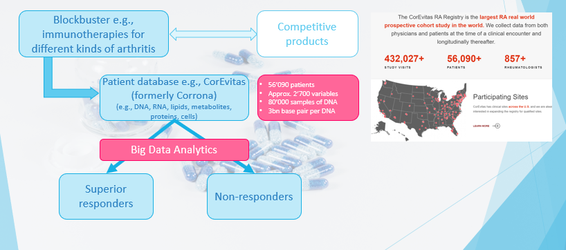
A blockbuster is a tremendously popular drug that generates at least annual revenues of more than $1 billion. Blockbusters address common diseases like diabetes, high blood pressure, common cancer types, or asthma. There are usually many competing products in the market.
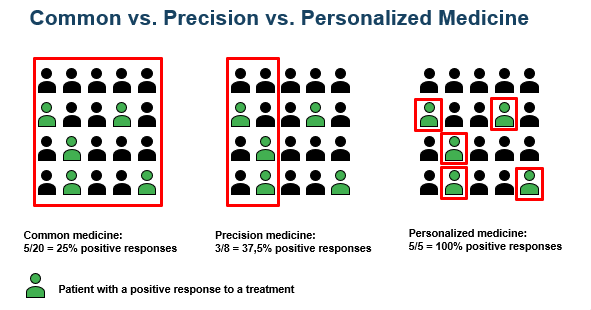
“Precision medicine” means that it is a treatment for groups of individuals who share certain characteristics that are responsive to that specific therapy (see graphic below).
For a better, i.e., a differentiation to other drugs, and for more specific targeting and marketing of the product, the patient groups that respond superior regarding its disease suppression are determined. The goal is the same as in every marketing analytics project. Data used are so-called real-world data (RWD), i.e., data of treated patients and not from clinical trials.
The main methods are supervised learning methods because we have a desired output value. Besides the common methods of regression / logistic regression, support vector machines, and random forest, today, with larger amounts of data, deep learning algorithms like convolutional neural networks (CNN) are applied. CNN often outperforms the other methods.
3. Predicting heart failure in mobile health
Heart failure typically leads to emergency or hospital admission. And with an aging population, the percentage of heart failure in the population is expected to increase.
People that suffer heart failure usually have pre-existing illnesses. So, it is not uncommon that telemedicine systems are used to monitor and consult a patient, and mobile health data like blood pressure, body weight, or heart rate are collected and transmitted.
Most prediction and prevention systems are based on fixed rules, e.g., when specific measurements are beyond a pre-defined threshold, the patient is alerted. It is self-explanatory that such a predictive system has a high number of false alerts, i.e., false positives.
Because an alert leads mostly to hospital admission, too many false alerts lead to increased health costs and deteriorate the patient’s confidence in the prediction. Eventually, she or he will stop following the recommendation for medical help.
So, based on baseline data of the patient like age, gender, smoker or not, pacemaker or not but also measurements of sodium, potassium or hemoglobin concentrations in the blood, and monitored characteristics like heart rate, body weight, (systolic and diastolic) blood pressure, or questionnaire answers about the well-being, or physical activities, a classifier based on Naïve Bayes has been finally developed.
The false alerts decreased by 73%, with an AUC (“area under the curve”) of about 70%.
4. Mental illness prediction, diagnosis, and treatment
It is estimated that at least 10% of the global population has a mental disorder. Economic losses caused by mental illness sum up to nearly $10 trillion. Mental disorders include, amongst others, anxiety, depression, substance use disorder, e.g., opioid, bipolar disorder, schizophrenia, or eating disorders.
So, the detection of mental disorders and intervention as early as possible is critical. There are two main approaches: apps for consumers that detect diseases and tools for psychiatrists to support diagnostics.
The apps for consumers are typically conversational chatbots enhanced with machine learning algorithms. The app analyzes the spoken language of the consumer, and recommendations for help are given. As the recommendations must be based on scientific evidence, the interaction and response of proposals and the individual language pattern must be predicted as accurately as possible.
The methods applied vary. The first step is almost always sentiment analysis. In simpler models, random forest and Naïve Bayes are used. These models are outperformed tremendously by neural networks with up to three hidden layers.
5. Research publication and database scanning for biomarkers of stroke
Stroke is one of the main reasons for disability and death. The lifetime risk of an adult person is about 25% of having once a stroke. But stroke is a very heterogeneous disorder. So, having individualized pre-stroke and post-stroke care is crucial for the success of a cure.
To determine this individualized care, the person’s phenotype, i.e., observable characteristics of a person should be chosen. And this is usually achieved by biomarkers. A so-called biomarker is a measurable data point such that the patients can be stratified. Examples are disease severity scores, lifestyle characteristics, or genomic properties.
There are many known biomarkers already published or in databases. Also, there are daily many hundreds of scientific publications about the detection of biomarkers for all the different diseases.
Research is enormously expensive and time-critical to prevent a disorder. So, biotech companies need to understand the most effective and efficient corresponding biomarkers for a particular disease. The amount of information is so gigantic that this cannot be done manually.
Data science helps in the development of sophisticated NLP algorithms to find relevant biomarkers in databases and publications. Besides understanding the content if such a biomarker is relevant for a particular type of stroke, a judgment of the published results’ quality must be achieved. This is a highly complex task overall.
6. 3D Bioprinting
Bioprinting is another hot topic in the biotechnology field. Based on a digital blueprint, the printer uses cells and natural or synthetic biomaterials — also called bioinks — to print layer-by-layer living tissues like skin, organs, blood vessels, or bones.
Instead of depending on organ donations, they can be produced in printers more ethically and cost-effectively. Also, drug tests are performed on the synthetic build tissue than with animal or human testing. The whole technology is still in early maturity due to its high complexity. One of the most essential parts to cope with this complexity of printing is data science.
The printing process and quality depend on numerous factors like the properties of the bioinks, which have inherent variabilities, or the various printing parameters. For example, to increase the success of getting usable output and thus, optimize the printing process, Bayesian optimization is applied.
The printing speed is a key component in the process. Siamese network models are deployed to determine the optimized speed. To detect material, i.e., tissue defects, convolutional neural networks are applied to images from the layer-by-layer tissue.
There are many more applications during the pre-production, production, and post-production process, but these three examples already show the complexity and advanced models needed. In my opinion, this field is one of the most exciting ones in biotechnology for data scientists.
7. Personalized therapy in ovarian cancer treatment
“Personalized” means that a treatment matched with the needs of one single individual is applied (see graphic above). Medical treatments are more and more based on the individualized characteristics of a patient.
These properties are disease subtypes, personal patient risks, health prognosis, and molecular and behavioral biomarkers. We have seen above that a biomarker is any measurable data point such that the patients can be stratified. Based on that data, the best individualized treatment for a single patient is determined.
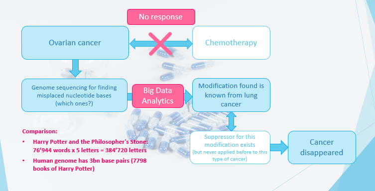
For one patient with ovarian cancer, the usual chemotherapy was not effective. So, one decided to perform genome sequencing to find the misplaced nucleotide bases that cause this cancer. With big data analytics, one found the modification amongst the 3 billion base pairs of a human, which corresponds to the number of words of 7798 books of Harry Potter’s “The Philosopher’s Stone.”
Methods applied are usually so-called covariance models, often combined with a classifier like random forest. Interestingly, this modification was known from lung cancer, where a drug exists but not from ovarian cancer. So, the treatment for lung cancer was applied, and the patient recovered.
8. Supply chain optimization
The production of drugs needs time, especially today’s high-tech cures based on specific substances and production methods. Also, the whole processes are broken down into many different steps, and several of them are outsourced to specialist providers.
We see this currently with the COVID-19 vaccine production. The vaccine inventors deliver the blueprint, and the production is in plants of companies specialized in sterile production. The vaccine is delivered in tanks to companies that do the filling in small doses under clinical conditions, and finally, another company makes the supply.
Further, drugs can be stored only for a limited time and often under special storage conditions, e.g., in a cold storage room.
The whole planning, from having the right input substances available at the right time, having the adequate production capacity, and finally, the proper amount of drugs stored for serving the demand, is a highly complex system. And this must be managed for hundreds and thousands of therapies, each with its specific conditions.
Computational methods are essential for managing this complexity. For example, the selection of the optimal partner companies in the production process is done by supervised learning like support vector machines.
Dynamic demand forecasting often relies on so-called support vector regression, and the production optimization itself deploy neural networks.
Conclusion
It is highly fascinating what modern technology and science can achieve today. It unfolds the most considerable value in combination with data science.
Method-wise, we see that supervised learning methods — random forest, Naïve Bayes, and support vector machines are often used, reinforcement learning, NLP, and deep learning are dominating.
Further, computational methods to cope with high dimensional data and search like principal component analysis and covariance models are needed.
Working on the frontier of innovation requires knowledge in particular topics like Bayesian optimization, convolutional neural networks, or Siamese networks.
The most significant entry barrier to this field is the topic-specific knowledge, thus understanding the (raw) data. The fastest path becoming familiar with is reading scientific publications and each expression that is not known, diligently to look up. When working in that field, you need to speak in the words of the experts.
Only then you can have an enormous impact as a data scientist. But this is also the most rewarding aspect.
I could never have more impact with my work than in the life sciences and biotechnology industry.
Do you like my story? Here you can find more.
I’m a part-time Amazon delivery driver. Here’s how we cheat to get around the strict rules.
I’m a part-time Amazon delivery driver. Here’s how we cheat to get around the strict rules and constant monitoring.
“We’ve created a workaround to game the system,” says one Amazon driver, who eats lunch while driving and has had to pee in water bottles.

By Jenny Powers
Jay (not his real name) has worked as a part-time driver delivering packages for Amazon in rural Michigan since 2019. He spoke anonymously out of concern for losing his position. His identity has been verified by Insider.
I started working part time as a driver for Amazon in 2019 after seeing an online classified ad. I enjoy travel and figured I could use a few extra bucks, so I applied.
My starting pay was $16 an hour. For my one-year anniversary, I got an increase of $0.25 an hour. Recently, drivers received a COVID-19 bonus — part-timers like me received $150.
It’s no secret that Amazon contracts the bulk of their deliveries through third-party delivery service providers (DSPs), so while I exclusively deliver Amazon packages and wear branded clothing with their logo on it, I don’t actually work for Amazon.
I like the DSP I work for and I’m thankful for the job, but Amazon’s constant need to implement new rules is frustrating and has resulted in a lot of turnover at my workplace.
There are around 25 to 30 full-time drivers, and usually the same number of weekend drivers floating around. This is partly due to the higher turnover of part-timers. My best estimate is there are 30 to 40 new drivers since last year.
It’s like a never-ending revolving door where every time I come in, there’s a new face.
Amazon preaches safety, safety, safety, and while that’s a great narrative for the media, behind the scenes it’s another story.
There’s a lot of pressure on the DSPs to perform well otherwise they risk getting their contract pulled, and this pressure winds up trickling down to us drivers.
In the name of safety, Amazon keeps tabs on us by tracking everything, but what it really does is create more pressure.
They monitor everything — from whether we’re wearing our seat belts to acceleration, braking, cornering, reversing, and even things like touching our screens while in motion through an app called Mentor.
The app can either be downloaded on our mobile phones or a phone provided by our DSP, which is what I opted for because I don’t like the idea of having a tracker on my personal phone.
At the end of each shift, which is typically between nine and 11 hours long, the app generates a score based on how well we drove. The highest score is 850.
When I started nearly two years ago, if you got a 550 you were fine, but not anymore. Now they want you to be in the high 700’s.
I used to have a 550, but now I’m more like a 750, which is basically the lowest score Amazon will allow without the DSP getting into trouble.
The problem is your score can take a hit for things completely out of your control.
For instance, if a kid runs into the street chasing their soccer ball and you’re forced to hit the brakes unexpectedly, that goes against your score. If a deer darts out in front of your van and you swerve to avoid an accident, that goes against your score, too. If you’re driving and your GPS suddenly goes down and you touch the screen to get back on track — boom, that’s another infraction. What else are we supposed to do in these situations?
I’ve never been in an accident, but these types of instances can drag a driver’s score down, and the bottom line is everything comes down to your score.
My DSP doesn’t want to jeopardize their business, so we’ve created a workaround to game the system.
If a driver’s scores start to suffer, our supervisor will tell us to log into the app at the beginning of our shift and then hand our phone over to a driver who typically scores high to take it out on their route. Problem solved.
I drive a rental van as opposed to an official Amazon vehicle, which I prefer because those can’t go over 70 MPH, not that I speed on anything.
If I’m told I have to get a camera in my van, I can tell you I probably won’t continue to work there. I don’t need to be under constant surveillance all day, even if it’s under the guise of safety.
From the moment we arrive at work, we’ve got to get our hustle on.
Once we arrive at the lot, we have to personally conduct a 60-point check on our vehicles before we get assigned to our routes, issued packets, and sent out in waves to our hub to pick up our packages. Some examples of things we need to check each shift are whether our wiper fluid is topped off, is our vehicle missing a gas cap, does our reverse camera work, and our tires for balding, pressure, and tread depth.
The hub is like a giant bee’s nest with everyone weaving in and out because we need to scan every package before loading our vehicle. Then we’ve got to move fast to ensure we can actually deliver everything on our route by 10 p.m. which is Amazon’s requirement.
I average about 150 packages and 130 stops per shift and about 30% to 40% more between peak season, which runs from October through December. During the peak, Amazon gives part-time drivers like me a $150 season bonus.
I’ve got a rural route most of the time, so the last thing I want is to be out here on some country road with no street lights delivering packages after dark.
We do get electronic notifications to take two 15-minute breaks during our shifts and a lunch break, but I always dismiss the notices and just eat while I’m driving — which is a no-no, but it’s really the only way to get the job done on time and not have to return any undelivered packages back to the hub.
The DSP gets penalized for returning packages, although I don’t know what the threshold is. I’m sure there’s an allowance built in for this as it’s just not safe to leave packages at some addresses, but my guess is the DSP gets penalized if too many are brought back.
I’m not proud to admit it, but I’ve peed in a bottle to save time on my route.
It’s partly by choice, part necessity. Working on these country routes, it can sometimes take as long as 20 minutes for me to find a fast-food restaurant or gas station, and I just don’t have that kind of time.
If there are four miles between houses and no one’s around, I might be able to pee on a country road, but more often than not, it’s a bottle in the van.
I rarely had to do this when I worked for UPS because they do so many commercial deliveries — I was always relatively close to a business where I could use the facilities.
Even on the days I do manage to finish early, it’s almost a guarantee I’ll get sent back out to help a driver on another route, which isn’t ideal because all I want to do is get home at that point.
There’s been a lot of talk about unionizing lately but personally, I’m not a big fan of unions. I feel like in the 1940s-50s they were beneficial, but now it’s just a big, greedy power grab.
When I worked as a temp driver at UPS, I wasn’t eligible for any benefits due to my part-time status, but I was still required to pay union dues.
One of the biggest issues between Amazon and its drivers is that the people making all the rules are sitting inside offices and not behind the wheel.
So more often than not, the rules being implemented are counterintuitive to what it actually takes to do our job safely and efficiently.
Amazon prides itself on getting driver safety under control, but then puts demands in place that force us to circumvent the system.
In a statement to Insider, an Amazon spokesperson said: We support drivers taking the time they need to take breaks in between stops and provide a list within the Amazon Delivery app to see nearby restroom facilities and gas stations. Drivers have built-in time on their route to take breaks and use the restroom. In fact, the app alerts them when it’s time for a break. We work closely with DSPs to set realistic expectations that do not place undue pressure on them or their drivers. We use sophisticated technology that plans routes to be completed within a specified time, taking into account numerous factors such as package volume, address complexity, and appropriate time for breaks. In fact, more than 75% of drivers complete their routes under the planned time by 30 minutes or more. Whether it’s state-of-the art safety technology in our vans, driver-safety training programs, or continuous improvements within our mapping and routing technology, we have invested tens of millions of dollars in safety mechanisms across our network, and regularly communicate safety best practices to drivers.
For more great stories, visit Insider’s homepage.
How to process a DataFrame with millions of rows in seconds
How to process a DataFrame with millions of rows in seconds
Yet another Python library for Data Analysis that You Should Know About — and no, I am not talking about Spark or Dask
Big Data Analysis in Python is having its renaissance. It all started with NumPy, which is also one of the building blocks behind the tool I am presenting in this article.
In 2006, Big Data was a topic that was slowly gaining traction, especially with the release of Hadoop. Pandas followed soon after with its DataFrames. 2014 was the year when Big Data became mainstream, also Apache Spark was released that year. In 2018 came Dask and other libraries for data analytics in Python.
Each month I find a new Data Analytics tool, which I am eager to learn. It is a worthy investment of spending an hour or two on tutorials as it can save you a lot of time in the long run. It’s also important to keep in touch with the latest tech.
While you might expect that this article will be about Dask you are wrong. I found another Python library for data analysis that you should know about.
Like Python, it is equally important that you become proficient in SQL. In case you aren’t familiar with it, and you have some money to spare, check out this course: Master SQL, the core language for Big Data analysis.
Big Data Analysis in Python is having its renaissance
In case you’ve missed my article about another Data Analytics tool:
Meet Vaex
Vaex is a high-performance Python library for lazy Out-of-Core DataFrames (similar to Pandas), to visualize and explore big tabular datasets.
It can calculate basic statistics for more than a billion rows per second. It supports multiple visualizations allowing interactive exploration of big data.
What’s the difference between Vaex and Dask?
Vaex is not similar to Dask but is similar to Dask DataFrames, which are built on top pandas DataFrames. This means that Dask inherits pandas issues, like high memory usage. This is not the case Vaex.
Vaex doesn’t make DataFrame copies so it can process bigger DataFrame on machines with less main memory.
Both Vaex and Dask use lazy processing. The only difference is that Vaex calculates the field when needed, wherewith Dask we need to explicitly use the compute function.
Data needs to be in HDF5 or Apache Arrow format to take full advantage of Vaex.
How to install Vaex?
To install Vaex is as simple as installing any other Python package:
pip install vaex
Let’s take Vaex to a test drive
Let’s create a pandas DataFrame with 1 million rows and 1000 columns to create a big data file.
import vaex
import pandas as pd
import numpy as npn_rows = 1000000
n_cols = 1000
df = pd.DataFrame(np.random.randint(0, 100, size=(n_rows, n_cols)), columns=['col%d' % i for i in range(n_cols)])df.head()

How much main memory does this DataFrame use?
df.info(memory_usage='deep')

Let’s save it to disk so that we can read it later with Vaex.
file_path = 'big_file.csv'
df.to_csv(file_path, index=False)
We wouldn’t gain much by reading the whole CSV directly with Vaex as the speed would be similar to pandas. Both need approximately 85 seconds on my laptop.
We need to convert the CSV to HDF5 (the Hierarchical Data Format version 5) to see the benefit with Vaex. Vaex has a function for conversion, which even supports files bigger than the main memory by converting smaller chunks.
If you cannot open a big file with pandas, because of memory constraints, you can covert it to HDF5 and process it with Vaex.
dv = vaex.from_csv(file_path, convert=True, chunk_size=5_000_000)
This function creates an HDF5 file and persists it to disk.
What’s the datatype of dv?
type(dv)# output
vaex.hdf5.dataset.Hdf5MemoryMapped
Now, let’s read the 7.5 GB dataset with Vaex — We wouldn’t need to read it again as we already have it in dv variable. This is just to test the speed.
dv = vaex.open('big_file.csv.hdf5')
Vaex needed less than 1 second to execute the command above. But Vaex didn’t actually read the file, because of lazy loading, right?
Let’s force to read it by calculating a sum of col1.
suma = dv.col1.sum()
suma# Output
# array(49486599)
I was really surprised by this one. Vaex needed less than 1 second to calculate the sum. How is that possible?
Opening such data is instantaneous regardless of the file size on disk. Vaex will just memory-map the data instead of reading it in memory. This is the optimal way of working with large datasets that are larger than available RAM.
Plotting
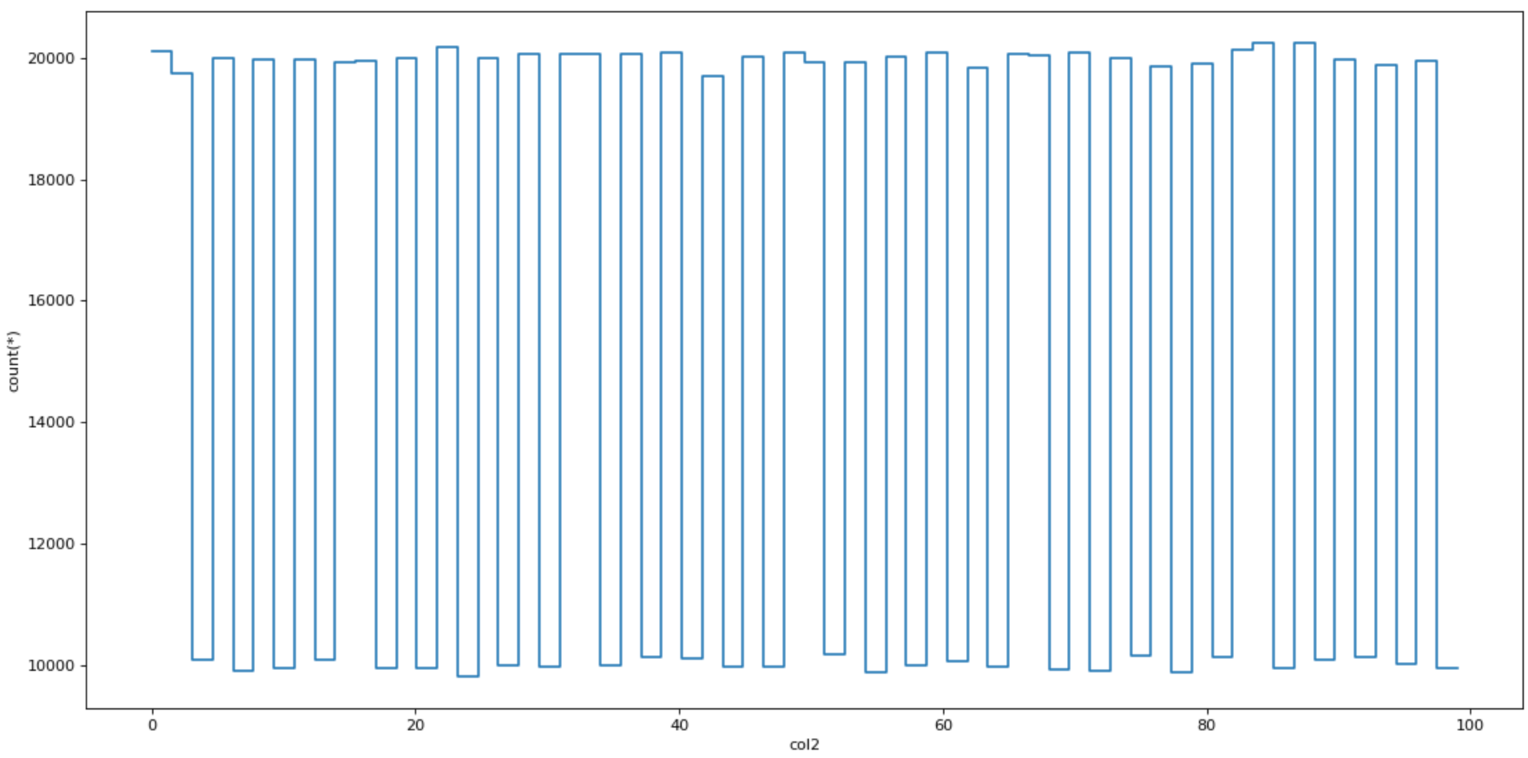
Vaex is also fast when plotting data. It has special plotting functions plot1d, plot2d and plot2d_contour.
dv.plot1d(dv.col2, figsize=(14, 7))
Virtual columns
Vaex creates a virtual column when adding a new column, — a column that doesn’t take the main memory as it is computed on the fly.
dv['col1_plus_col2'] = dv.col1 + dv.col2
dv['col1_plus_col2']

Efficient filtering
Vaex won’t create DataFrame copies when filtering data, which is much more memory efficient.
dvv = dv[dv.col1 > 90]
Aggregations
Aggregations work slightly differently than in pandas, but more importantly, they are blazingly fast.
Let’s add a binary virtual column where col1 ≥ 50.
dv['col1_50'] = dv.col1 >= 50
Vaex combines group by and aggregation in a single command. The command below groups data by the “col1_50” column and calculates the sum of the col3 column.
dv_group = dv.groupby(dv['col1_50'], agg=vaex.agg.sum(dv['col3']))
dv_group

Joins
Vaex joins data without making memory copies, which saves the main memory. Pandas users will be familiar with the join function:
dv_join = dv.join(dv_group, on=’col1_50')
Conclusion
In the end, you might ask: Should we simply switch from pandas to Vaex? The answer is a big NO.
Pandas is still the best tool for data analysis in Python. It has well-supported functions for the most common data analysis tasks.
When it comes to bigger files, pandas might not be the fastest tool. This is a great place for Vaex to jump in.
Vaex is a tool you should add to your Data Analytics toolbox.
When working on an analysis task where pandas is too slow or simply crashes, pull Vaex out of your toolbox, filter out the most important entries and continue the analysis with pandas.
Before you go
- How To Create Date Series in SQL [Article]- Free skill tests for Data Scientists & Machine Learning Engineers- Advance your Career in Cybersecurity (60% off) [Course]- Become a Cloud Developer using Microsoft Azure [Course]- Master SQL, the core language for Big Data analysis [Course]
Some of the links above are affiliate links and if you go through them to make a purchase I’ll earn a commission. Keep in mind that I link courses because of their quality and not because of the commission I receive from your purchases.
Follow me on Twitter, where I regularly tweet about Data Science and Machine Learning.
Build and Run a Docker Container for your Machine Learning Model
Build and Run a Docker Container for your Machine Learning Model
A quick and easy build of a Docker container with a simple machine learning model

The idea of this article is to do a quick and easy build of a Docker container with a simple machine learning model and run it. Before reading this article, do not hesitate to read Why use Docker for Machine Learning and Quick Install and First Use of Docker.
In order to start building a Docker container for a machine learning model, let’s consider three files: Dockerfile, train.py, inference.py.
You can find all files on GitHub.
The train.py is a python script that ingest and normalize EEG data in a csv file (train.csv) and train two models to classify the data (using scikit-learn). The script saves two models: Linear Discriminant Analysis (clf_lda) and Neural Networks multi-layer perceptron (clf_NN).
The inference.py will be called to perform batch inference by loading the two models that has been previously created. The application will normalize new EEG data coming from a csv file (test.csv), perform inference on the dataset and print the classification accuracy and predictions.
Let’s create a simple Dockerfile with the jupyter/scipy-notebook image as our base image. We need to install joblib to allow serialization and deserialization of our trained model. We copy the train.csv, test.csv, train.py and inference.py files into the image. Then, we run train.py which will fit and serialize the machine learning models as part of our image build process which provide several advantages such as the ability to debug at the beginning of the process, use Docker Image ID for keeping track or use different versions.
In order to build the image, we run the following command in our terminal:
docker build -t docker-ml-model -f Dockerfile .
The output is the following:

It’s time to perform the inference on new data (test.csv):
docker run docker-ml-model python3 inference.py
The output is the following:

We can do a few things that can improve our containerization experience. We can for example bind a host directory in the container using WORKDIR in the Dockerfile:
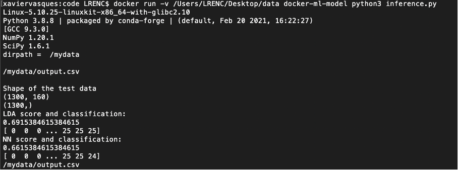
In inference.py, we can decide for example to save an output.csv file with the X_test data in it:
When you build it and run it you should be able to see the output.csv file in /mydata :
We can also add the VOLUME instruction in the Dockerfile resulting in an image that will create a new mount point:
With the name that we specify, the VOLUME instruction creates a mount point which is tagged as holding externally mounted volume from native host or other containers where we find the data we want to process.
For the future of your developments, it can be necessary to set environment variables from the beginning, just once at the build time, for persisting the trained model and maybe add additional data or metadata to a specific location. The advantage of setting environment variables is to avoid the hard code of the necessary paths all over your code and to better share your work with others on an agreed directory structure.
Let’s take another example, with a new Dockerfile:
We need to add the environment variables to train.py:
and inference.py:
What’s Next ?
The goal was to produce quick and easy steps to build a Docker container with a simple machine learning model. Building is as simple as doing a docker build -t my-docker-image ..
From this step, we can start the deployment of our models which will be much simpler and removing the fear to publish and scale your machine learning model. The next step is to produce a workflow with a CI/CD tool (Continuous Integration/Continuous Delivery) such as Jenkins. Thanks to this approach, it will be possible to build and serve anywhere a docker container and expose a REST API so that external stakeholders can consume it. If you are training a deep learning model that needs high computational needs, you can move your containers to high performance computing servers or any platform of your choice such as on premises, private or public cloud. The idea is that you can scale your model but also create resilient deployment as you can scale the container across regions/availability zones.
I hope you can see the great simplicity and flexibility containers provide. By containerizing your machine/deep learning application, you can make it visible to the world. The next step is to deploy it in the cloud and expose it. At certain points in time, you will need to orchestrate, monitor and scale your containers to serve millions of users with the help of technologies such as Red Hat OpenShift, a Kubernetes distribution.
Sources
https://docs.docker.com/engine/reference/builder/
