One of the often-overlooked parts of sequence generation in natural language processing (NLP) is how we select our output tokens — otherwise known as decoding.
You may be thinking — we select a token/word/character based on the probability of each token assigned by our model.
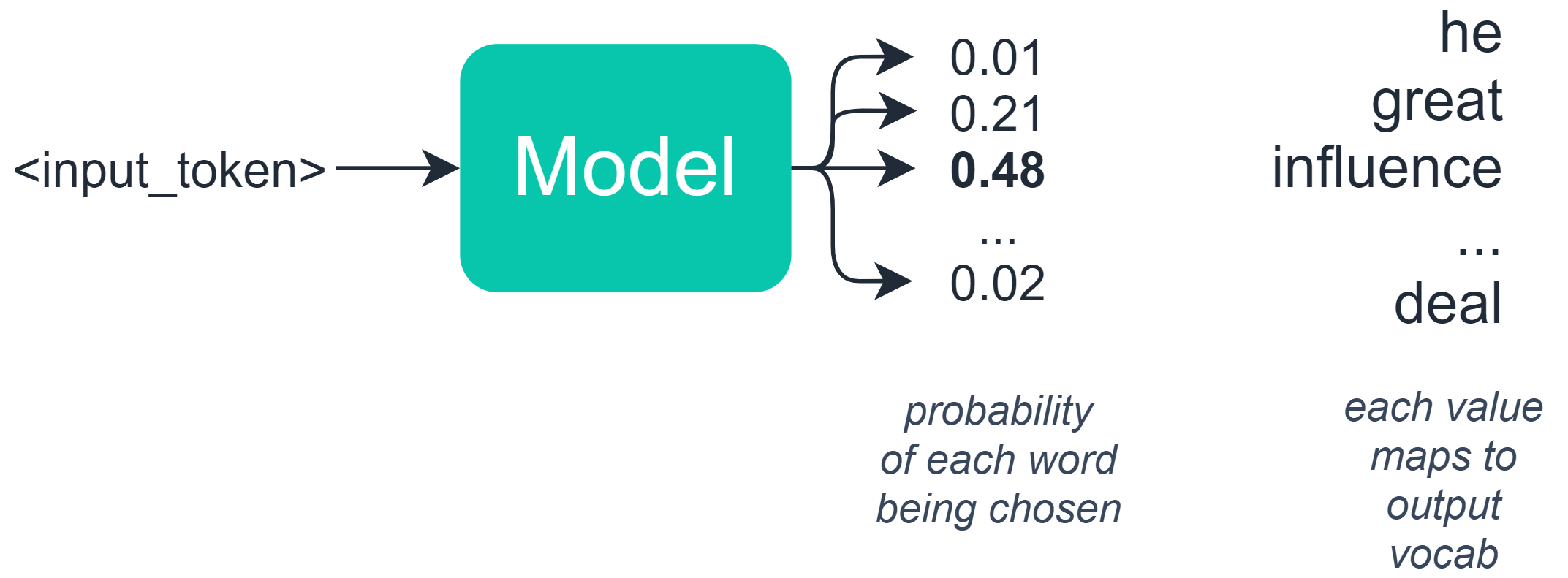
This is half-true — in language-based tasks, we typically build a model which outputs a set of probabilities to an array where each value in that array represents the probability of a specific word/token.
At this point, it might seem logical to select the token with the highest probability? Well, not really — this can create some unforeseen consequences — as we will see soon.
When we are selecting a token in machine-generated text, we have a few alternative methods for performing this decode — and options for modifying the exact behavior too.
In this article we will explore three different methods for selecting our output token, these are:
> Greedy Decoding> Random Sampling> Beam Search
It’s pretty important to understand how each of these works — often-times in language applications, the solution to a poor output can be a simple switch between these four methods.
If you’d prefer video, I cover all three methods here too:
I’ve included a notebook for testing each of these methods with GPT-2 here.
Greedy Decoding
The simplest option we have is greedy decoding. This takes our list of potential outputs and the probability distribution already calculated — and chooses the option with the highest probability (argmax).
It would seem that this is entirely logical — and in many cases, it works perfectly well. However, for longer sequences, this can cause some problems.
If you have ever seen an output like this:
The default text is what we fed into the model — the green text has been generated.
This is most likely due to the greedy decoding method getting stuck on a particular word or sentence and repetitively assigning these sets of words the highest probability again and again.
Random Sampling
The next option we have is random sampling. Much like before we have our potential outputs and their probability distribution.
Random sampling chooses the next word based on these probabilities — so in our example, we might have the following words and probability distribution:
Random sampling allows us to randomly choose a word based on its probability previously assigned by the model
We would have a 48% chance of the model selecting ‘influence’, a 21% chance of it choosing ‘great’, and so on.
This solves our problem of getting stuck in a repeating loop of the same words because we add randomness to our predictions.
However, this introduces a different problem — we will often find that this approach can be too random and lacks coherence:
So on one side, we have greedy search which is too strict for generating text — on the other we have random sampling which produces wonderful gibberish.
We need to find something that does a little of both.
Beam Search
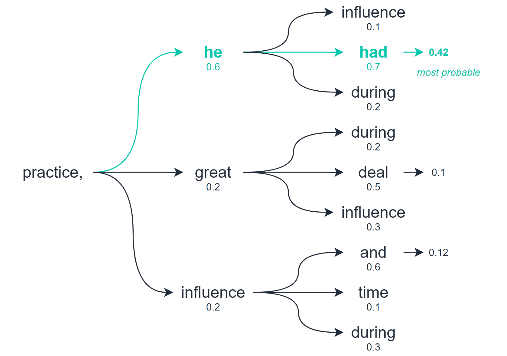
Beam search allows us to explore multiple levels of our output before selecting the best option.
Beam search, as a whole the ‘practice, he had’ scored higher than any other potential path
So whereas greedy decoding and random sampling calculate the best option based on the very next word/token only — beam search checks for multiple word/tokens into the future and assesses the quality of all of these tokens combined.
From this search, we will return multiple potential output sequences — the number of options we consider is the number of ‘beams’ we search with.
However, because we are now back to ranking sequences and selecting the most probable — beam search can cause our text generation to again degrade into repetitive sequences:
So, to counteract this, we increase the decoding temperature — which controls the amount of randomness in the outputs. The default temperature is 1.0 — pushing this to a slightly higher value of 1.2 makes a huge difference:
With these modifications, we have a peculiar but nonetheless coherent output.
That’s it for this summary of text generation decoding methods!
I hope you’ve enjoyed the article, let me know if you have any questions or suggestions via Twitter or in the comments below.
Thanks for reading!
If you’re interested in learning how to set up a text generation model in Python, I wrote this short article covering how here:
조건부 확률 이론은 종종 특정 수학적 문제에 대한 독특하고 흥미로운 솔루션으로 이어집니다.복잡한 확률 문제를 비교적 간단하게 해결할 수있을 때 흥분과 불신이 섞여 있습니다.조건부 확률과 실험 결과를 중심으로 한 유명한 통계 시나리오 인 Gambler ‘s Ruin Problem의 경우는 확실히 해당됩니다.이 문제에 대해 훨씬 더 매력적인 것은 그 구조가 조건부 확률을 넘어 무작위 변수 및 분포로 확장된다는 것입니다. 특히 흥미로운 특성을 가진 고유 한 마르코프 체인의 적용으로 확장됩니다.
초등학교피강도 문제는 불확실한 결과에 대한 수학적 설명을 기반으로합니다.초등학교 통계는 복잡한 시나리오를 이해하고 정리를 사용하여 불확실한 결과의 확률을 결정하는 데 사용할 수있는 도구 세트를 제공합니다.도박꾼의 파멸 문제를 해결하는 것은 우리가 매일해야하는 일이 아니지만, 그 구조를 이해하면 불확실성에 뿌리를 둔 상황에 접근 할 때 비판적이고 수학적 사고 방식을 개발하는 데 도움이됩니다.
엔ote :이 게시물은 독자가 미적분과 선형 대수에 대한 노출을 필요로하는 기초 확률과 통계 이론을 이해해야합니다.또한 독자가 Markov 체인에 대한 몇 가지 기본 지식을 가지고 있다고 가정합니다.
문제 설명
가장 기본적인 형태의 Gambler ‘s Ruin Problem은 두 명의 도박꾼으로 구성됩니다.ㅏ과비확률 론적 게임을 여러 번하고 있습니다.게임을 할 때마다 확률이 있습니다피(0 & lt;피& lt;1) 그 도박꾼ㅏ도박꾼에게 이길 것이다비.마찬가지로 기본 확률 공리를 사용하여 도박꾼이비이길 것입니다 1-피.각 도박꾼은 또한 베팅 할 수있는 금액을 제한하는 초기 자산을 가지고 있습니다.총 결합 부는 다음과 같이 표시됩니다.케이그리고 도박꾼ㅏ초기 재산은나는, 이는 도박꾼이비초기 재산이k-나.부는 긍정적이어야합니다.이 문제에 적용하는 마지막 조건은 두 도박꾼이 둘 중 한 명이 초기 재산을 모두 잃어 더 이상 플레이 할 수 없을 때까지 무기한 플레이한다는 것입니다.
그 도박꾼을 상상해보십시오ㅏ의 초기 재산나는정수 달러 금액이며 각 게임은 1 달러로 진행됩니다.그건 도박꾼이ㅏ적어도 플레이해야 할 것입니다나는그들의 부를 0으로 떨어 뜨리는 게임.그들이 각 게임에서 1 달러를 이길 확률은피, 게임이 두 도박꾼 모두에게 공평하다면 1/2이됩니다.만약피& gt;1/2, 도박꾼ㅏ체계적인 이점이 있고피& lt;1/2 이후 도박꾼ㅏ체계적인 단점이 있습니다.일련의 게임은 두 가지 결과로만 끝날 수 있습니다. 도박꾼ㅏ풍부한케이달러 (도박꾼비모든 돈을 잃었습니다) 또는 도박꾼ㅏ0 달러의 부 (도박꾼비모든 부가 있습니다).분석의 주요 초점은 도박꾼이ㅏ풍부한으로 끝날 것입니다케이0 달러 대신 달러.결과에 관계없이 도박꾼 중 한 명이 재정적으로파멸, 따라서 이름도박꾼의 폐허.
문제 해결책
위에서 설명한 동일한 구조를 계속 사용하여 이제 확률을 결정하려고합니다.aᵢ그 도박꾼ㅏ끝날 것이다케이그들이 시작한 것을 감안할 때 달러나는불화.단순함을 위해 여기에 추가 가정을 추가하겠습니다. 모든 게임은 동일하고 독립적입니다.도박꾼이 새로운 게임을 할 때마다 가장 최근 게임의 결과에 따라 각 도박꾼의 초기 재산이 다른 Gambler ‘s Ruin 문제의 새로운 반복으로 해석 될 수 있습니다.수학적으로 우리는 도박꾼으로 끝나는 게임의 각 순서를 생각할 수 있습니다.ㅏ갖는제이어디 달러제이= 0,…,케이.확률 도박꾼ㅏ특정 시퀀스가 발생하면 승리합니다.aⱼ.도박꾼으로 끝나는 모든 시퀀스ㅏ갖는케이달러는 그들이 이겼 음을 의미하므로aₖ= 1.마찬가지로 도박꾼으로 끝나는 모든 시퀀스ㅏ0 달러는 그들이 파멸에 빠졌다는 것을 의미하므로ㅏ₀ = 0.우리는 모든 값에 대한 확률을 결정하는 데 관심이 있습니다.i = 1,…, k-1.
이벤트 표기법을 사용하여ㅏ₁ 도박꾼이ㅏ게임 1에서 승리합니다.비₁은 도박꾼이비게임 1에서 승리합니다. 이벤트W도박꾼이ㅏ결국케이0 달러로 끝나기 전에 달러.이 이벤트가 발생할 확률은 조건부 확률의 속성을 사용하여 도출 할 수 있습니다.
조건부 확률을 사용한 승리 확률
그 도박꾼을 감안할 때ㅏ로 시작나는그들이 이길 확률은P (W) = aᵢ.도박꾼이라면ㅏ첫 번째 게임에서 1 달러를 획득하면 재산이i +1. 첫 게임에서 1 달러를 잃으면 재산은나는-1. 전체 시퀀스에서 이길 확률은 첫 번째 게임에서 이겼는지 여부에 따라 달라집니다.이 논리를 이전 방정식에 적용하면 게임마다 1 달러를 이길 확률과 도박꾼의 재산이 주어진 시퀀스에서 이길 조건부 확률에 의존하는 전체 게임 시퀀스에서 이길 확률의 표현을 알 수 있습니다.
문제 표기법을 사용한 승리 확률
도박꾼의 부ㅏ주어진 시점에서 도박꾼의 총 초기 자산과 0 사이에 차이가 있습니다.즉, 주어진i =1, … ,k-1, 우리는 모든 가능한 값을 연결할 수 있습니다나는구하기 위해 위의 방정식에k-인접한 값을 기반으로 승리 확률을 결정하는 1 방정식나는.기초 대수를 사용하여 이러한 방정식을 단일 공식으로 단순화 할 수있는 표준화 된 형식으로 집계 할 수 있습니다.이 공식은 각 게임에서 승리 할 확률 간의 근본적인 관계를 지정합니다.피, 두 도박꾼의 총 초기 자산케이, 그리고 1 달러의 재산이 주어질 때 이길 확률ㅏ₁.일단 우리가 결정하면ㅏ₁, 우리는 모든 것을 반복적으로 반복 할 수 있습니다.k-확률을 도출하려면 1aᵢ가능한 모든 값에 대해나는.
Fundamental relation
이제 우리는 두 가지 가능성을 고려할 것입니다 : 공정한 게임과 불공정 한 게임,피위의 방정식에 연결합니다.공정한 게임에서피= 1 / 2, 방정식의 오른쪽에있는 지수의 밑은 (1-피) /피= 1.그런 다음 전체 방정식을 다음과 같이 단순화 할 수 있습니다. 1-ㅏ₁ = (케이– 1)ㅏ₁, 재정렬 가능ㅏ₁ = 1 /케이.다른 값에 대한 승리 확률을 결정하는 모든 이전 방정식을 반복하면나는,공정한 게임을위한 일반적인 해결책에 도달했습니다.
공정한 게임을위한 솔루션
위의 방정식은 놀라운 결과입니다. 게임이 공정하다는 점을 감안할 때 도박꾼이ㅏ끝날 것이다케이0 달러로 끝나기 전의 달러는 초기 자산과 같습니다.나는두 도박꾼의 총 재산으로 나눈케이.
만약피두 명의 도박꾼 중 한 명이 체계적인 이점을 가지고 있기 때문에 게임이 불공평합니다.우리는 유사하게 가치에 의존하는 일반적인 해결책을 도출 할 수 있습니다.피그리고 부 매개 변수.
불공정 한 게임에 대한 해결책
노트: 독자가 일반적인 솔루션에 도달하기 위해 수학적 증명을 배우는 데 관심이 있다면 마지막에있는 참고 문헌을 참조하십시오.
랜덤 변수의 시퀀스엑스이산 시간 간격에 의해 정의 된 다른 시점을 나타내는 것은 확률 적 프로세스라고 할 수 있습니다.프로세스의 첫 번째 랜덤 변수는초기 상태,프로세스의 나머지 랜덤 변수는 시간에 각 프로세스의 상태를 정의합니다.엔.마르코프 체인은 미래 상태의 조건부 분포가 현재 상태에만 의존하는 특정 종류의 확률 적 프로세스입니다.즉, 조건부 분포엑스시간에n + j…에 대한j & gt;0시간의 프로세스 상태에만 의존엔, 이전 상태가 아닌엔– 1.다음 표기법을 사용하여이를 수학적으로 표현할 수 있습니다.
마르코프 사슬
마르코프 사슬은한정된특정 시점에 발생할 수있는 상태 수가 무한이 아닌 경우체인을 고려하십시오케이상태.시간에서의 상태 확률 분포n + 1특정 값을 취하는제이당시의 상태로엔로 알려져 있습니다전환 분포마르코프 사슬의.분포가 매번 동일한 경우 이러한 분포는 고정 된 것으로 간주됩니다.엔.표기법을 사용할 수 있습니다.pᵢⱼ이러한 분포를 나타냅니다.
고정 전이 분포
서로 다른 값의 총 수pᵢⱼ가능한 상태의 총 수에 따라 걸릴 수 있습니다.케이, 우리는케이으로케이매트릭스피마르코프 사슬의 전이 행렬로 알려져 있습니다.
전환 매트릭스
전이 행렬에는 고유하게 만드는 중요한 속성이 있습니다.행렬의 모든 요소는 확률을 나타내므로 모든 요소는 양수입니다.각 행은 이전 상태의 값이 주어 졌을 때 다음 상태의 전체 조건부 분포를 나타내므로 각 행의 값은 1이됩니다. 전이 행렬을 사용하여 확률 계산을 간단한 방법으로 여러 단계로 확장 할 수 있습니다.즉, 우리는 Markov 체인이 상태에서 이동할 확률을 계산할 수 있습니다.나는상태로제이여러 단계로미디엄전환 매트릭스를 취함으로써피의 힘에미디엄.즉,m 단계 전이 행렬피ᵐ는 체인의 모든 단계 범위 사이에서 특정 상태의 확률을 계산하는 데 사용할 수 있습니다.
대각선이있는 전이 행렬이있는 경우pᵢᵢ1과 같으면 상태나는간주됩니다흡수 상태.마르코프 사슬이 흡수 상태가되면 그 후에는 다른 상태로 들어갈 수 없습니다.또 다른 흥미로운 특성은 Markov 체인에 하나 이상의 흡수 상태가있는 경우 체인이 결국 이러한 상태 중 하나로 흡수된다는 것입니다.
시간 1에서 Markov 체인의 시작 부분에서 요소가 체인이 각 상태에있을 확률을 나타내는 벡터를 지정할 수 있습니다.이것은초기 확률 벡터V. We can determine the marginal distribution of the chain at any time 엔초기 확률 벡터를 곱하여V전환 매트릭스에 의해피의 힘에엔-1. 예를 들어, 우리는 다음 식으로 시간 2에서 체인의 한계 분포를 찾을 수 있습니다.vP.
A special case occurs when a probability vector multiplied by the transition matrix is equal to itself: vP=V.이것이 발생하면 확률 벡터를고정 분포마르코프 체인을 위해.
도박꾼의 폐허 마르코프 사슬
Markov 체인의 이론적 프레임 워크를 사용하여 이제 이러한 개념을 Gambler ‘s Ruin 문제에 적용 할 수 있습니다.우리가 이것을 할 수 있다는 사실은 확률과 통계 이론이 얼마나 얽혀 있는지 보여줍니다.처음에는 기본 확률 공리에서 파생 된 조건부 확률 정리만을 사용하여 문제를 구성했습니다.이제 문제를 더욱 공식화하고 Markov 체인을 사용하여 더 많은 구조를 제공 할 수 있습니다.추상적 개념을 취하고 다양한 도구를 사용하여 분석하고 확장하는 과정은 통계의 마법을 강조합니다.
갬블러의 파멸 문제는 본질적으로 갬블러가A 어떤 시점에서든 기본 구조를 결정합니다.즉, 언제든지엔, 도박꾼ㅏ가질 수있다i wealth, where i 또한 시간의 체인 상태를 나타냅니다.엔. When the gambler reaches either 0 wealth or k 부, 체인은 흡수 상태로 이동하고 더 이상 게임을하지 않습니다.
If the chain moves into any of the remaining k – 1 states 1, … , k – 1, a game is played again where the probability that gambler ㅏ이길거야피determines the marginal distribution of the state at that specific point in time. The transition matrix has two absorbing states. The first row corresponds to the scenario when gambler ㅏhas 0 wealth and the elements of the row are (1, 0, … , 0). Likewise, the last row of the transition matrix corresponds to the scenario when gambler ㅏhas reached 케이부와 요소는 (0,…, 1)입니다.다른 모든 행에 대해i, 요소는 좌표가있는 항에 대해 모두 0입니다.i – 1 and i + 1, which have values 1 – p and 피 respectively.
Gambler’s Ruin transition matrix
We can also determine the probabilities of states in multiple steps using the m-step transition matrixPᵐ. As 미디엄goes to infinity, the m-step matrix converges but the stationary distributions are not unique. The limit matrix of 피ᵐ에는 첫 번째 및 마지막 열을 제외하고 모두 0이 있습니다.마지막 열에는 모든 확률이 포함됩니다.aᵢ that gambler A 끝날 것이다케이그들이 시작한 것을 감안할 때 달러i dollars, while the first column contains all the respective complements of aᵢ.Since the stationary distributions are not unique, that means that all of the probabilities belong to the absorbing states.
Gambler’s Ruin limit matrix
This last point is especially important because it confirms our initial logical sequence of steps when deriving the solution formulas to the Gambler’s Ruin. In other words, we are able to derive a general formula for the problem as a whole because the stochastic processes (sequence of games) that occur in the problem converge to one of two absorbing states: gambler A 멀리 걸어케이dollars or gamblerㅏwalks away with 0 dollars. 무한히 많은 게임을 할 수 있지만 Markov 체인의 전이 행렬이 두 고정 분포로 수렴하기 때문에이 두 이벤트 중 하나가 발생할 확률을 결정할 수 있습니다.
결론
The Gambler’s Ruin Problem is a great example of how you can take a complex situation and derive a simple general structure from it using statistical tools. It might be difficult to believe that, given a fair game, the probability that someone will win enough games to claim the total wealth of both players is determined by their initial wealth and the total wealth. This is known not only at the beginning of the sequence, but also at each step. Using Markov chains, we can determine the same probabilities between any sequences of games using the transition matrix and the probability vector at the initial state. Consider this, the conclusion that we came to in the first section of this post was enhanced by use of an additional concept. Applying different perspectives to the same problem can open the door to insightful analysis. This is the power of theoretical statistical thinking.
Conditional probability theory often leads to unique and interesting solutions to certain mathematical problems. There is a mix of excitement and disbelief when a complex probabilistic problem can be solved in a relatively simply manner. This is certainly the case with the Gambler’s Ruin Problem, a famous statistical scenario centered around conditional probabilities and experimental outcomes. What is possibly even more fascinating about this problem is that its structure extends beyond conditional probability into random variables and distributions, particularly as an application of unique Markov chains with interesting properties.
Elementary probability problems are based on mathematical descriptions of uncertain outcomes. Elementary statistics gives us a set of tools that we can use to determine probabilities of uncertain outcomes using theorems as well as demystifying complex scenarios. Solving the Gambler’s Ruin Problem is not a task that we must do on a daily basis, but understanding its structure helps us develop a critical and mathematical mindset when approaching situations rooted in uncertainty.
Note: This post requires that the reader understands elementary probability and statistical theory, which itself requires exposure to both calculus and linear algebra. It is also assumed that the reader has some basic knowledge on Markov chains.
Problem Statement
The Gambler’s Ruin Problem in its most basic form consists of two gamblers A and B who are playing a probabilistic game multiple times against each other. Every time the game is played, there is a probability p (0 < p < 1) that gambler A will win against gambler B. Likewise, using basic probability axioms, the probability that gambler B will win is 1 – p. Each gambler also has an initial wealth that limits how much they can bet. The total combined wealth is denoted by k and gambler A has an initial wealth denoted by i, which implies that gambler B has an initial wealth of k – i.Wealth is required to be positive. The last condition we apply to this problem is that both gamblers will play indefinitely until one of them has lost all their initial wealth and thus cannot play anymore.
Imagine that gambler A’s initial wealth i is an integer dollar amount and that each game is played for one dollar. That means that gambler A will have to play at least i games for their wealth to drop to zero. The probability that they win one dollar in each game is p, which will be equal to 1/2 if the game is fair for both gamblers. If p > 1/2, then gambler A has a systematic advantage and if p < 1/2 then gambler A has a systematic disadvantage. The series of games can only end in two outcomes: gambler A has a wealth of k dollars (gambler B lost all their money), or gambler A has a wealth of 0 dollars (gambler B has all the wealth). The main focus of the analysis is to determine the probability that gambler A will end up with a wealth of k dollars instead of 0 dollars. Regardless of the outcome, one of the gamblers will end up in financial ruin, hence the name Gambler’s Ruin.
Problem Solution
Continuing with the same structure outlined above, we now want to determine the probability aᵢ that gambler A will end up with k dollars given that they started out with i dollars. For the sake of simplicity, we will add an additional assumption here: all games are identical and independent. Every time the gamblers play a new game, it can be interpreted as a new iteration of the Gambler’s Ruin problem where the initial wealth of each gambler are different, depending on the outcome of the most recent game. Mathematically, we can think of each sequence of games that ends in gambler A having j dollars where j = 0, … , k. The probability gambler A wins given that a specific sequence occurs is aⱼ. Any sequence that ends in gambler A having k dollars means that they won, so aₖ=1. Likewise, any sequence than ends in gambler A having 0 dollars means that they are in ruin so a₀=0. We are interested in determining the probabilities for all values of i=1, … , k – 1.
Using event notation, we can denote A₁ as the event that gambler A wins game 1. Similarly, B₁ is the event that gambler B wins game 1. The event W occurs when gambler A ends up with k dollars before they end up with 0 dollars. The probability that this event occurs can be derived using properties of conditional probability.
Probability of winning using conditional probabilities
Given that gambler A starts with i dollars, the probability that they win is P(W)=aᵢ. If gambler A wins one dollar in the first game, then their wealth becomes i+1. If they lost one dollar in the first game, their fortune becomes i – 1. The probability that they win the entire sequence will then depend on whether they won they won the first game. When we apply this logic to the previous equation, we know have an expression of the probability of winning the entire sequence of games that depends on the probability of winning one dollar each game and the conditional probabilities of winning the sequence given the gamblers wealth.
Probability of winning using problem notation
The wealth of gambler A at any given point in time varies between the total initial wealth of both gamblers and zero. In other words, given i=1, … , k – 1, we can plug in all possible values of i into the equation above to obtain k – 1 equations that determine the probability of winning based on adjacent values of i. We can use elementary algebra to aggregate these equations into a standardized format that can be simplified into a single formula. This formula specifies a fundamental relation between the probability of winning each game p, the total initial wealth of both gamblers k, and the probability of winning given a wealth of one dollar a₁. Once we have determined a₁, we can iteratively loop through all k – 1 to derive the probability aᵢ for all possible values of i.
Fundamental relation
We will now consider two possibilities: a fair game and an unfair game, which depends on the value of p that we plug into the equation above. In a fair game, where p=1/2, the base of the exponent in the right side of the equation can be simplified to (1 – p)/p=1. We can then simplify the entire equation as follows: 1 – a₁=(k – 1)a₁, which can be rearranged to a₁=1/k. If we iterate over all previous equations that determine the probabilities of winning for different values of i, we arrive at a general solution for fair games.
Solution for a fair game
The equation above is a remarkable result: given that the game is fair, the probability that gambler A will end up with k dollars before they end up with zero dollars is equal to their initial wealth i divided by the total wealth of both gamblers k.
If p is not equal to 1/2 the game is unfair, as one of the two gamblers has a systematic advantage. We can similarly derive a general solution which depends on the value of p and the wealth parameters.
Solution to an unfair game
Note: If the reader is interested in learning the mathematical proofs to arrive at the general solutions, consult the references at the end.
A sequence of random variables X that represent different points in time defined by discrete time intervals can be referred to as a stochastic process. The first random variable in the process is known as the initial state, and the rest of the random variables in the process define the state of each process at time n. Markov chains are a specific kind of stochastic process where conditional distributions of future states depend only on the present state. That is, the conditional distribution of X at time n + j for j > 0 depends only on the state of the process at time n, not on any of the earlier states up to n – 1. We can express this mathematically using the following notation.
Markov chain
A Markov chain is finite if the number of states that can occur at any point in time is noninfinite. Consider a chain with k states. The probability distribution of a state at time n+1 taking a specific value j given the state at time n is known as the transition distribution of the Markov chain. These distributions are considered stationary if the distribution is the same for each time n. We can use the notation pᵢⱼ to denote these distributions.
Stationary transition distributions
The total number of different values that pᵢⱼ can take depends on the total number of possible states k, which we can arrange in a k by k matrix P known as the transition matrix of the Markov chain.
Transition matrix
Transition matrices have important properties that make them unique. Since every element of the matrix represents a probability, all elements are positive. Since each row represents the entire conditional distribution of the next state given the value of the previous state, the values in each row sum to 1. We can extend the probability calculations to multiple steps in a straightforward way by using the transition matrix. That is, we can calculate the probability that the Markov chain will move from a state i to a state j in multiple steps m by taking the transition matrix P to the power of m. That is, the m-step transition matrixPᵐ can be used to calculate the probabilities of specific states between any range of steps in the chain.
If we have a transition matrix where any of the diagonals pᵢᵢ are equal to 1, then the state i is considered an absorbing state. Once a Markov chain goes into an absorbing state, it cannot go into any other state thereafter. Another interesting property is that if a Markov chain has one or more absorbing states, the chain will be absorbed into one of those states eventually.
At the beginning of the Markov chain at time 1, we can specify a vector whose elements represent the probabilities that the chain will be in each state. This is known as the initial probability vector v. We can determine the marginal distribution of the chain at any time n by multiplying the initial probability vector v by the transition matrix P to the power of n – 1. For example, we can find the marginal distribution of the chain at time 2 by the expression vP.
A special case occurs when a probability vector multiplied by the transition matrix is equal to itself: vP=v. When this occurs, we call the probability vector the stationary distribution for the Markov chain.
Gambler’s Ruin Markov Chains
Using the theoretical framework for Markov chains, we can now apply these concepts to the Gambler’s Ruin problem. The fact that we are able to do this shows how intertwined probability and statistical theory can be. We initially framed the problem using exclusively conditional probability theorems derived from the basic probability axioms. Now we can formalize the problem even further and give it more structure using Markov chains. The process of taking an abstract concept and using various tools to analyze it and expand it underlines the magic of statistics.
The Gambler’s Ruin problem is essentially a Markov chain where the sequence of wealth amounts that gambler A has at any point in time determines the underlying structure. That is, at any point in time n, gambler A can have i wealth, where i also represents the state of the chain at time n. When the gambler reaches either 0 wealth or k wealth, the chain has moved into an absorbing state and no more games are played.
If the chain moves into any of the remaining k – 1 states 1, … , k – 1, a game is played again where the probability that gambler A will win p determines the marginal distribution of the state at that specific point in time. The transition matrix has two absorbing states. The first row corresponds to the scenario when gambler A has 0 wealth and the elements of the row are (1, 0, … , 0). Likewise, the last row of the transition matrix corresponds to the scenario when gambler A has reached k wealth and the elements are (0, … , 1). For every other row i, the elements are all zero expect for the terms with coordinates i – 1 and i + 1, which have values 1 – p and p respectively.
Gambler’s Ruin transition matrix
We can also determine the probabilities of states in multiple steps using the m-step transition matrixPᵐ. As m goes to infinity, the m-step matrix converges but the stationary distributions are not unique. The limit matrix of Pᵐ has all zeroes except in its first and last columns. The last column contains all probabilities aᵢ that gambler A will end up with k dollars given that they started out with i dollars, while the first column contains all the respective complements of aᵢ. Since the stationary distributions are not unique, that means that all of the probabilities belong to the absorbing states.
Gambler’s Ruin limit matrix
This last point is especially important because it confirms our initial logical sequence of steps when deriving the solution formulas to the Gambler’s Ruin. In other words, we are able to derive a general formula for the problem as a whole because the stochastic processes (sequence of games) that occur in the problem converge to one of two absorbing states: gambler A walks away with k dollars or gambler A walks away with 0 dollars. Even though infinitely many games can be played, we can still determine the probability that either one of these two events occur because the transition matrix of the Markov chain converges to both stationary distributions.
Conclusion
The Gambler’s Ruin Problem is a great example of how you can take a complex situation and derive a simple general structure from it using statistical tools. It might be difficult to believe that, given a fair game, the probability that someone will win enough games to claim the total wealth of both players is determined by their initial wealth and the total wealth. This is known not only at the beginning of the sequence, but also at each step. Using Markov chains, we can determine the same probabilities between any sequences of games using the transition matrix and the probability vector at the initial state. Consider this, the conclusion that we came to in the first section of this post was enhanced by use of an additional concept. Applying different perspectives to the same problem can open the door to insightful analysis. This is the power of theoretical statistical thinking.