저는 항상 도시지도를 좋아했고 몇 주 전에 나만의 예술적 버전을 만들기로 결정했습니다.인터넷 검색을 한 후이 놀라운 사실을 발견했습니다.지도 시간작성자프랭크 세발 로스.매혹적이고 편리한 튜토리얼이지만 더 자세하고 사실적인 청사진 맵을 선호합니다.그래서 나만의 버전을 만들기로 결정했습니다.이제 작은 파이썬 코드와 OpenStreetMap 데이터로 아름다운지도를 만드는 방법을 살펴 보겠습니다.
OSMnx 설치
우선, 우리는Python 설치가 있습니다.나는 사용하는 것이 좋습니다콘다깔끔한 작업 공간을 확보하기위한 가상 환경 (venv).또한 OpenStreetMap에서 공간 데이터를 다운로드 할 수있는 OSMnx Python 패키지를 사용할 것입니다.Venv를 만들고 두 개의 Conda 명령을 작성하기 만하면 OSMnx를 설치할 수 있습니다.
conda 구성-채널 앞에 추가 conda-forge
conda create -n ox --strict-channel-priority osmnx
Downloading street networks
OSMnx를 성공적으로 설치 한 후 코딩을 시작할 수 있습니다.가장 먼저해야 할 일은 데이터를 다운로드하는 것입니다.데이터 다운로드는 다양한 방법으로 수행 할 수 있습니다. 가장 쉬운 방법 중 하나는graph_from_place ().
베를린 거리 네트워크 다운로드
graph_from_place ()여러 매개 변수가 있습니다.장소OpenStreetMaps에서 데이터를 검색하는 데 사용할 쿼리입니다.보유 _ 모두다른 요소와 연결되어 있지 않더라도 우리에게 모든 거리를 줄 것입니다.단순화반환 된 그래프를 약간 정리하고network_type얻을 거리 네트워크의 유형을 지정하십시오.
나는 검색을 찾고있다모두가능한 데이터를 사용하지만 드라이브 도로 만 다운로드 할 수도 있습니다.드라이브, 또는산책.
또 다른 가능성은graph_from_point ()GPS 좌표를 지정할 수 있습니다.이 옵션은 일반적인 이름을 가진 장소와 같은 여러 경우에 더 편리하며 더 정확합니다.사용dist그래프 중심의이 수 미터 내에있는 노드 만 유지할 수 있습니다.
마드리드 거리 네트워크 다운로드
또한 마드리드 나 베를린과 같은 더 큰 장소에서 데이터를 다운로드하는 경우 모든 정보를 검색하기 위해 조금 기다려야한다는 점을 고려해야합니다.
데이터 압축 풀기 및 채색
양자 모두graph_from_place ()과graph_from_point ()다음과 같이 목록에 압축을 풀고 저장할 수있는 MultiDiGraph를 반환합니다.Frank Ceballos 튜토리얼.
이 지점에 도달하면 데이터를 반복하고 색상을 지정하기 만하면됩니다.색상을 지정하고 조정할 수 있습니다.선폭거리 기지길이.
그러나 특정 도로를 식별하고 다르게 색상을 지정할 수도 있습니다.
내 예에서는 다음 색상으로 만 colourMap.py Gist를 사용하고 있습니다.
색상 =“# a6a6a6”
색상 =“# 676767”
색상 =“# 454545”
색상 =“#bdbdbd”
색상 =“# d5d5d5”
색상 =“#ffff”
그러나 취향에 맞는 새로운지도를 만들기 위해 색상이나 조건을 자유롭게 변경하십시오.
지도 플로팅 및 저장
마지막으로,지도를 그리는 데 남은 한 가지만 있으면됩니다.먼저지도의 중심을 식별해야합니다.중심이 될 GPS 좌표를 선택하십시오.그런 다음 테두리와 배경색을 추가하고bgcolor.북쪽,남쪽,동쪽과서쪽서쪽은 우리지도의 새로운 경계가 될 것입니다.이 좌표는 이러한 경계에서 이미지 기반을 자르고 더 큰지도를 원할 때 경계를 늘리면됩니다.다음을 사용하는 경우graph_from_point ()방법을 늘릴 필요가 있습니다dist당신의 필요에 따라 가치 기반.에 대한bgcolor청사진을 시뮬레이션하기 위해 파란색에서 진한 파란색 # 061529를 선택했지만 원하는대로 조정할 수 있습니다.
그런 다음지도를 플로팅하고 저장하기 만하면됩니다.나는 사용을 추천한다fig.tight_layout (pad = 0)서브 플롯이 잘 맞도록 플롯 매개 변수를 조정합니다.
결과
이 코드를 사용하여 다음 예제를 작성할 수 있지만 각 도시의 선 너비 또는 경계 제한과 같은 설정을 실행하는 것이 좋습니다.
마드리드 도시지도 — 포스터 크기
고려해야 할 한 가지 차이점graph_from_place ()과graph_from_point ()그것은graph_from_point ()주변에서 거리 데이터를 얻습니다.dist설정합니다.간단한지도를 원하는지 더 자세한지도를 원하는지에 따라 서로 교환 할 수 있습니다.마드리드 도시지도는graph_from_place ()베를린 도시지도는graph_from_point ().
베를린 시티지도
그 위에 포스터 크기 이미지를 원할 수도 있습니다.이를 달성하는 한 가지 쉬운 방법은무화과내부 속성ox.plot_graph ().무화과너비, 높이를 인치 단위로 조정할 수 있습니다.나는 보통 같은 더 큰 크기를 선택했습니다figsize = (27,40).
보너스 : 물 추가
OpenStreetMap에는 강 및 호수 또는 수로와 같은 기타 천연 수원의 데이터도 있습니다.다시 OSmnx를 사용하여이 데이터를 다운로드 할 수 있습니다.
천연 수원 다운로드
이전과 같은 방식으로이 데이터를 반복하고 색상을 지정할 수 있습니다.이 경우 # 72b1b1 또는 # 5dc1b9와 같은 파란색을 선호합니다.
마지막으로 그림을 저장하면됩니다.이 경우에는 테두리를 사용하지 않습니다.bbox내부plot_graph.그것은 당신이 놀 수있는 또 다른 것입니다.
강을 성공적으로 다운로드 한 후 두 이미지를 결합하면됩니다.약간의 Gimp 또는 Photoshop이 트릭을 수행 할 것입니다. 동일한 두 이미지를 만들어야합니다.fig_size또는 경계 제한,bbox,보다 쉬운 보간을 위해.
베를린 천연 수원
마무리
내가 추가하고 싶은 것은 도시 이름, GPS 좌표 및 국가 이름이 포함 된 텍스트입니다.한 번 더 Gimp 또는 Photoshop이 트릭을 수행합니다.
또한 물을 추가하면 일부 공간을 채우거나 바닷물과 같은 다른 수원을 칠해야합니다.강의 선은 일정하지 않지만 페인트 통 도구를 사용하여 이러한 간격을 채울 수 있습니다.
코드 및 결론
이러한지도를 만드는 코드는 내GitHub.자유롭게 사용 하시고 결과를 보여주세요 !!이 게시물을 좋아하고 다시 감사드립니다.프랭크 세발 로스및 Medium 커뮤니티.또한 포스터를 인쇄하고 싶다면 작은 가게를 열었습니다.Etsy내지도 제작과 함께.
I always liked city maps and a few weeks ago I decided to build my own artistic versions of it. After googling a little bit I discovered this incredible tutorial written by Frank Ceballos. It is a fascinating and handy tutorial, but I prefer a more detailed/realistic blueprint maps. Because of that, I decided to build my own version. So let’s see how we can create beautiful maps with a little python code and OpenStreetMap data.
Installing OSMnx
First of all, we need tohave a Python installation. I recommend using Conda and virtual environments (venv) for achieving a tidy workspace. Moreover, we are going to use OSMnx Python package that will let us download spatial data from OpenStreetMap. We can accomplish the creation of a venv and installing OSMnx just writing two Conda commands:
After successfully install OSMnx, we can start coding. The first thing we need to do is to download the data. Downloading the data can be achieved in different ways, one of the easiest ways is to use graph_from_place().
Downloading Berlin street network
graph_from_place()has several parameters. placeis the query that is going to be used in OpenStreetMaps to retrieving the data, retain_allwill give us all the streets even if they are not connected to other elements, simplifyclean a little bit the returned graph and network_typespecify what type of street network to get.
I am looking to retrieve allpossible data but you can also download only drive roads, using drive, or pedestrian pathways using walk.
Another possibility is to use graph_from_point()that allows us to specify a GPS coordinate. This option is more in handy in multiple cases, like places with common names, and gives us more precision. Using distwe can retain only those nodes within this many meters of the centre of the graph.
Downloading Madrid street network
Also, it is necessary to take into account that if you are downloading data from bigger places like Madrid or Berlin, you will need to wait a little bit in order to retrieve all the information.
Unpacking and colouring our data
Both graph_from_place() and graph_from_point() will return a MultiDiGraph that we can unpack and store in the list as shown in Frank Ceballos tutorial.
Reaching this point we just need to iterate over data and colour it. We can colour it and adjust linewidths base on street lengths.
But there is also the possibility of identifying certain roads and only colour them differently.
In my example, I am only using colourMap.py Gist with the following colours.
color = “#a6a6a6”
color = “#676767”
color = “#454545”
color = “#bdbdbd”
color = “#d5d5d5”
color = “#ffff”
But feel free of changing the colours or conditions in order to create new maps that suit your taste.
Plot and save the map
Finally, we only need one thing left that is plotting the map. First, we need to identify the centre of our map. Choose the GPS coordinates where you want to be the centre. Then we will add some borders and background colour, bgcolor. north, south, eastand westwest will be new borders of our map. This coordinates will crop the image base on these boundaries, just increase the boundaries in you want a bigger map. Take into account that if you are using graph_from_point() method you will need to increase the dist value base on your needs. For bgcolor I am choosing a blue a dark blue #061529, to simulate a blueprint, but again you can adjust this to your liking.
After that, we just need to plot and save the map. I recommend use fig.tight_layout(pad=0) to adjust the plot params so that subplots are nicely fit.
Results
Using this code we can build the following examples but I recommend that you tunning your settings like line widths or border limit for each city.
Madrid City Map — Poster size
One difference to take into account between graph_from_place() and graph_from_point() it is that graph_from_point() will obtain street data from the surroundings, base on the dist that you set. Depending on if you want a simple map or a more detailed one you can exchange between them. The Madrid city map has been created using graph_from_place() and the Berlin city map has been created using graph_from_point() .
Berlin City Map
On top of that perhaps you want a poster size image. One easy way to accomplish that is to set figsizeattribute inside ox.plot_graph() .figsize can adjust the width, height in inches. I usually chose a bigger size like figsize=(27,40) .
Bonus: Add Water
OpenStreetMap has also data from rivers and other natural water sources, like lakes or water canals. Again using OSmnx we can download this data.
Downloading natural water sources
In the same way as before we can iterate over this data and colour it. In this case, I prefer blue colours like #72b1b1 or #5dc1b9.
Finally, we just need to save the figure. In this case, I am not using any borders with bbox inside plot_graph . That’s another thing that you can play with.
After successfully downloading rivers and like we just need to join the two images. Just a little Gimp or Photoshop will do the trick, remember to create the two images with the same fig_size or limit borders, bbox , for easier interpolation.
Berlin natural water sources
Finishing touches
One thing that I like to add is a text with the name of the city, GPS coordinates and the country name. Once more Gimp or Photoshop will do the trick.
Also if you add water you will need to fill some spaces or paint other water sources, like seawater. The line with of the rivers is not constant but using the paint bucket tool you can fill those gaps.
Code and conclusions
The code for creating these maps is available on my GitHub. Feel free to use it and show me your results!! Hope you liked this post and again thanks to Frank Ceballos and the Medium community. Additionally, if any of you want to print some posters I opened a little store on Etsy with my map creations.
Thanks for reading me and sharing knowledge will guide us to better and incredible results!!
A Short Introduction to Reinforcement Learning (RL)
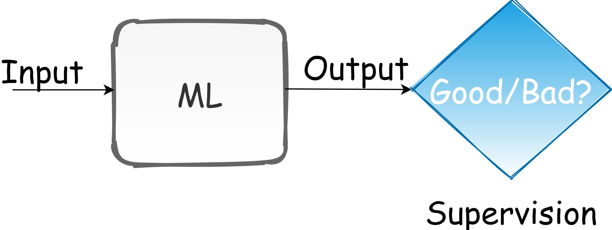
일반적인 기계 학습 접근 방식에는 세 가지 유형이 있습니다. 1) 학습 시스템이 레이블이 지정된 예를 기반으로 잠재 맵을 학습하는지도 학습, 2) 학습 시스템이 레이블이없는 예를 기반으로 데이터 배포를위한 모델을 설정하는 비지도 학습, 3) 강화 학습, 여기서의사 결정 시스템은 최적의 결정을 내릴 수 있도록 훈련됩니다.디자이너의 관점에서 모든 종류의 학습은 손실 함수에 의해 감독됩니다.감독의 출처는 인간에 의해 정의되어야합니다.이를 수행하는 한 가지 방법은 손실 함수입니다.
작성자의 이미지
감독 중디학습, 지상 실측 레이블이 제공됩니다.그러나 RL에서는 환경을 탐색하여 에이전트를 가르칩니다.에이전트가 과제를 해결하려는 세상을 디자인해야합니다.이 디자인은 RL과 관련이 있습니다.공식 RL 프레임 워크 정의는 [1]에 의해 제공됩니다.
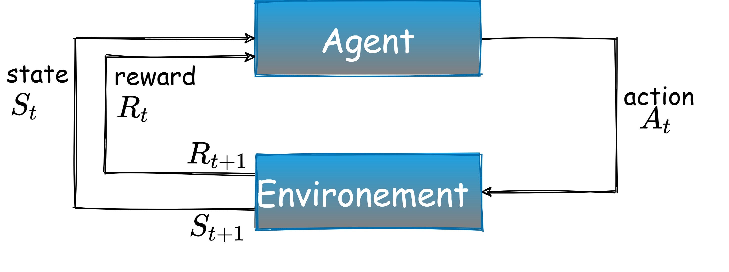
an에이전트에서 연기환경.모든 시점에서 에이전트는상태환경을 결정하고동작상태를 변경합니다.이러한 각 작업에 대해 에이전트는보상신호.에이전트의 역할은받은 총 보상을 극대화하는 것입니다.
RL 다이어그램 (저자 이미지)
그래서 어떻게 작동합니까?
RL은 시행 착오를 통해 순차적 인 의사 결정 문제를 해결하는 방법을 배우기위한 프레임 워크입니다.가끔 보상을 제공하는 세계의 오류.이것은 어떤 목표를 달성하기 위해 불확실한 환경에서 수행 할 일련의 작업을 경험을 통해 결정하는 작업입니다.행동 심리학에서 영감을받은 강화 학습 (RL)은이 문제에 대한 공식적인 틀을 제안합니다.인공 에이전트는 환경과 상호 작용하여 학습 할 수 있습니다.수집 된 경험을 사용하여 인공 에이전트는 누적 보상을 통해 주어진 일부 목표를 최적화 할 수 있습니다.이 접근법은 원칙적으로 과거 경험에 의존하는 모든 유형의 순차적 의사 결정 문제에 적용됩니다.환경은 확률적일 수 있으며 에이전트는 현재 상태에 대한 일부 정보 만 관찰 할 수 있습니다.
왜 깊이 들어가야합니까?
지난 몇 년 동안 RL은 도전적인 순차적 의사 결정 문제를 성공적으로 해결함으로써 점점 인기를 얻었습니다.이러한 성과 중 일부는 RL과 딥 러닝 기술의 조합 때문입니다.예를 들어 딥 RL 에이전트는 수천 개의 픽셀로 구성된 시각적 지각 입력으로부터 성공적으로 학습 할 수 있습니다 (Mnih et al., 2015/2013).
“AI에서 가장 흥미로운 분야 중 하나입니다.그것은 세계를 표현하고 이해하기 위해 심층 신경망의 힘과 능력을 합쳐서 세상을 행동하고 이해하는 능력과 결합하는 것입니다.”
이전에는 기계에 도달 할 수 없었던 광범위한 복잡한 의사 결정 작업을 해결했습니다.Deep RL은 의료, 로봇 공학, 스마트 그리드, 금융 등에서 많은 새로운 애플리케이션을 엽니 다.
RL의 유형
가치 기반: 상태 또는 상태-작업 값을 학습합니다.주에서 가장 좋은 행동을 선택하여 행동하십시오.탐험이 필요합니다.정책 기반: 상태를 행동으로 매핑하는 확률 적 정책 함수를 직접 학습합니다.샘플링 정책에 따라 행동하십시오.모델 기반: 세계의 모델을 배우고 모델을 사용하여 계획합니다.모델을 자주 업데이트하고 다시 계획하십시오.
수학적 배경
이제 우리는 “모델없는”접근 방식에 속하는 가치 기반 방법에 초점을 맞추고,보다 구체적으로 Q- 학습에 속하는 DQN 방법에 대해 논의 할 것입니다.이를 위해 필요한 수학적 배경을 빠르게 검토합니다.
어디이자형기대 값 연산자, 감마는 할인 계수,파이이다정책.그만큼최적의 기대 수익다음과 같이 정의됩니다.
최적의 V- 값 함수는 주어진 상태에서 예상되는 할인 된 보상입니다.에스에이전트는 정책을 따릅니다.파이 *그후에.
2.Q 값
관심있는 더 많은 기능이 있습니다.그중 하나는 품질 가치 기능입니다.
V- 기능과 유사하게 최적의큐값은 다음과 같이 지정됩니다.
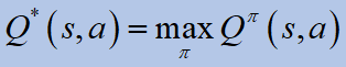
최적큐-value는 주어진 상태에있을 때 그리고 주어진 행동에 대해 예상되는 할인 된 수익입니다.ㅏ,에이전트는 정책을 따릅니다.파이 *그후에.최적의 정책은이 최적 값에서 직접 얻을 수 있습니다.
삼.장점 기능
마지막 두 기능을 연관시킬 수 있습니다.
행동이 얼마나 좋은지 설명합니다.ㅏ직접 정책을 따를 때 예상 수익과 비교됩니다.파이.
4.Bellman 방정식
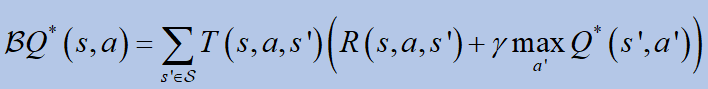
배우려면큐값, Bellman 방정식이 사용됩니다.독특한 솔루션을 약속합니다큐*:
어디비Bellman 연산자입니다.
최적의 가치를 약속하기 위해 : 상태-액션 쌍은 개별적으로 표현되고 모든 액션은 모든 상태에서 반복적으로 샘플링됩니다.
Q- 학습
정책을 벗어난 방법의 Q 학습은 주에서 행동을 취하고 학습하는 것의 가치를 배웁니다.큐가치와 세상에서 행동하는 방법을 선택합니다.상태-액션 값 함수를 정의합니다.에스,실행할 수 있는ㅏ, 및 팔로우파이.표 형식으로 표시됩니다.에 따르면큐에이전트는 모든 정책을 사용하여큐미래의 보상을 극대화합니다.큐직접 근사치큐*, 에이전트가 각 상태-작업 쌍을 계속 업데이트 할 때.
딥 러닝이 아닌 접근 방식의 경우이 Q 함수는 표일뿐입니다.
작성자의 이미지
이 표에서 각 요소는 보상 값이며, 훈련 중에 업데이트되어 정상 상태에서 할인 계수로 보상의 예상 값에 도달해야합니다.큐*값.실제 시나리오에서 가치 반복은 비현실적입니다.
Google의 이미지
에서브레이크 아웃 게임,상태는 화면 픽셀입니다. 이미지 크기 : 84×84, 연속 : 4 개 이미지, 회색 수준 : 256. 따라서큐-테이블은 :
언급하자면, 우주에는 10⁸² 원자가 있습니다.이것이 우리가 다음과 같은 문제를 해결해야하는 좋은 이유입니다.브레이크 아웃 게임심층 강화 학습에서…
DQN : Deep Q-Networks
우리는 신경망을 사용하여큐함수:
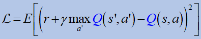
신경망은 함수 근사로 유용합니다.DQN은 Atari 게임에서 사용되었습니다.손실 함수에는 두 가지 Qs 함수가 있습니다.
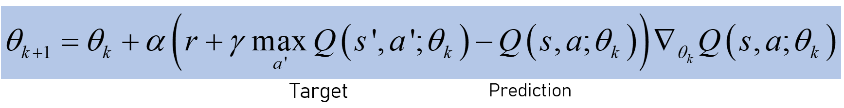
표적: 특정 상태에서 행동을 취할 때 예상되는 Q 값.예측: 실제로 그 행동을 취할 때 얻는 가치 (다음 단계에서 가치를 계산하고 총 손실을 최소화하는 것을 선택).
매개 변수 업데이트 :
가중치를 업데이트 할 때 대상도 변경됩니다.신경망의 일반화 / 외삽으로 인해 상태-행동 공간에 큰 오류가 발생합니다.따라서 Bellman 방정식은 w.p.1.이 업데이트 규칙으로 오류가 전파 될 수 있습니다 (느림 / 불안정 등).
DQN 알고리즘은 다양한 ATARI 게임에 대한 온라인 설정에서 강력한 성능을 얻을 수 있으며픽셀.불안정성을 제한하는 두 가지 경험적 방법 : 1. 대상의 매개 변수큐-network는 N 반복마다 업데이트됩니다.이렇게하면 불안정성이 빠르게 전파되는 것을 방지하고 분산 위험을 최소화합니다.경험 리플레이 메모리 트릭을 사용할 수 있습니다.
DQN 아키텍처 (MDPI : 경제학에서 심층 강화 학습 방법 및 응용 프로그램에 대한 포괄적 인 검토)
DQN 트릭 : 리플레이와 엡실론 탐욕스러운 경험
리플레이 체험
DQN에서는 CNN 아키텍처가 사용됩니다.비선형 함수를 사용한 Q- 값의 근사값은 안정적이지 않습니다.경험 리플레이 트릭에 따르면 모든 경험은 리플레이 메모리에 저장됩니다.네트워크를 훈련 할 때 가장 최근의 작업 대신 재생 메모리의 임의 샘플이 사용됩니다.즉, 에이전트는 기억 / 저장 경험 (상태 전환, 행동 및 보상)을 수집하고 훈련을위한 미니 배치를 만듭니다.
엡실론 탐욕 탐사
로큐기능 수렴큐*, 실제로 발견 한 첫 번째 효과적인 전략으로 해결됩니다.따라서 탐사는 탐욕 스럽습니다.탐색하는 효과적인 방법은 확률이 “엡실론”이고 그렇지 않은 경우 (1- 엡실론), 탐욕스러운 행동 (가장 높은 Q 값)을 가진 무작위 행동을 선택하는 것입니다.경험은 엡실론 탐욕 정책에 의해 수집됩니다.
DDQN : Double Deep Q-Networks
의 최대 연산자큐-학습은 행동을 선택하고 평가하기 위해 동일한 값을 사용합니다.이는 과대 평가 된 값 (노이즈 또는 부정확 한 경우)을 선택하여 과도하게 낙관적 인 값을 추정하게 만듭니다.DDQN에는 각각 별도의 네트워크가 있습니다.큐.따라서 두 개의 신경망이 있습니다.현재 가중치로 얻은 값에 따라 정책이 여전히 선택되는 편향을 줄이는 데 도움이됩니다.
견인 신경망,큐각 기능 :
이제 손실 함수는 다음과 같이 제공됩니다.
Deep Q-Networks 결투
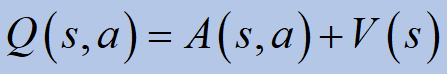
큐포함이점(ㅏ)값 (V) 그 상태에 있습니다.ㅏ조치를 취하는 이점으로 일찍 정의ㅏ주에스다른 모든 가능한 작업 및 상태 중에서.당신이 취하고 자하는 모든 행동이“아주 좋은”것이라면, 우리는 그것이 얼마나 더 나은지 알고 싶습니다.
결투 네트워크는 두 개의 개별 추정치를 나타냅니다. 하나는 상태 값 함수를위한 것이고 다른 하나는 상태 의존적 행동 이점 함수를위한 것입니다.코드 예제를 더 읽으려면듀얼 딥 큐 네트워크게시크리스 윤.
요약
우리는 강화 학습에 대한 일반적인 소개와이를 딥 러닝 맥락에 넣을 동기 부여와 함께 가치 기반 방법의 Q- 러닝을 제시했습니다.수학적 배경, DQN, DDQN, 몇 가지 트릭 및 결투 DQN이 탐구되었습니다.
저자 정보
Barak Or는 B.Sc.(2016), M.Sc.(2018) 항공 우주 공학 학위 및 B.A.Technion, Israel Institute of Technology에서 경제 및 경영학 박사 (2016, Cum Laude).그는 Qualcomm (2019–2020)에서 주로 기계 학습 및 신호 처리 알고리즘을 다루었습니다.Barak은 현재 그의 Ph.D.하이파 대학교에서.그의 연구 관심 분야는 센서 융합, 내비게이션, 기계 학습 및 추정 이론입니다.
Value-based Methods in Deep Reinforcement Learning
Deep Reinforcement learning has been a rising field in the last few years. A good approach to start with is the value-based method, where the state (or state-action) values are learned. In this post, a comprehensive review is provided where we focus on Q-learning and its extensions.
A Short Introduction to Reinforcement Learning (RL)
There are three types of common machine learning approaches: 1) supervised learning, where a learning system learns a latent map based on labeled examples, 2) unsupervised learning, where a learning system establishes a model for data distribution based on unlabeled examples, and 3) Reinforcement Learning, where a decision-making system is trained to make optimal decisions. From the designer’s point-of-view, all kinds of learning are supervised by a loss function. The sources of supervision must be defined by humans. One way to do this is by the loss function.
Image by author
In supervised learning, the ground truth label is provided. But, in RL, we teach an agent by exploring the environment. We should design the world where the agent is trying to solve a task. This design is related to RL. A formal RL framework definition is given by [1]
an agent acting in an environment. At every point in time, the agent observes the state of the environment and decides on an action that changes the state. For each such action, the agent is given a reward signal. The agent’s role is to maximize the total received reward.
RL Diagram (image by author)
So, how it works?
RL is a framework for learning to solve sequential decision-making problems by trial & error in a world that provides occasional rewards. This is the task of deciding, from experience, the sequence of actions to perform in an uncertain environment to achieve some goals. Inspired by behavioral psychology, reinforcement learning (RL) proposes a formal framework for this problem. An artificial agent may learn by interacting with its environment. Using the experience gathered, the artificial agent can optimize some objectives given via cumulative rewards. This approach applies in principle to any type of sequential decision-making problem relying on past experience. The environment may be stochastic, the agent may only observe partial information about the current state, etc.
Why go deep?
Over the past few years, RL has become increasingly popular due to its success in addressing challenging sequential decision-making problems. Several of these achievements are due to the combination of RL with deep learning techniques. For instance, a deep RL agent can successfully learn from visual perceptual inputs made up of thousands of pixels (Mnih et al., 2015 / 2013).
“One of the most exciting fields in AI. It’s merging the power and the capabilities of deep neural networks to represent and comprehend the world with the ability to act and then understanding the world”.
It has solved a wide range of complex decision-making tasks that were previously out of reach for a machine. Deep RL opens up many new applications in healthcare, robotics, smart grids, finance, and more.
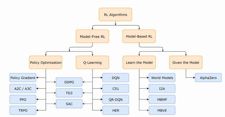
Types of RL
Value-Based: learn the state or state-action value. Act by choosing the best action in the state. Exploration is necessary. Policy-Based: learn directly the stochastic policy function that maps state to action. Act by sampling policy. Model-Based: learn the model of the world, then plan using the model. Update and re-plan the model often.
Mathematical background
We now focus on the value-based method, which belongs to “model-free” approaches, and more specifically, we will discuss the DQN method, which belongs to Q-learning. For that, we quickly review some necessary mathematical background.
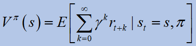
An RL agent goal is to find a policy such that it optimizes the expected return (V-value function):
where Eis the expected value operator, gamma is the discount factor, and pi isa policy. The optimal expected return is defined as:
The optimal V-value function is the expected discounted reward when in a given statesthe agent follows the policypi* thereafter.
2. Q value
There are more functions of interest. One of them is the Quality Value function:
Similarly to the V-function, the optimal Q value is given by:
The optimal Q-value is the expected discounted return when in a given state s and for a given action, a,the agent follows the policy pi* thereafter. The optimal policy can be obtained directly from this optimal value:
3. Advantage function
We can relate between the last two functions:
It describes “how good” the action ais, compared to the expected return when following direct policy pi.
4. Bellman equation
To learn the Q value, the Bellman equation is used. It promises a unique solution Q*:
where B is the Bellman operator:
To promise optimal value: state-action pairs are represented discretely, and all actions are repeatedly sampled in all states.
Q-Learning
Q learning in an off-policy method learns the value of taking action in a state and learning Q value and choosing how to act in the world. We define state-action value function: an expected return when starting in s, performing a, and following pi. Represented in a tabulated form. According to Q learning, the agent uses any policy to estimate Q that maximizes the future reward. Q directly approximates Q*, when the agent keeps updating each state-action pair.
For non-deep learning approaches, this Q function is just a table:
Image by author
In this table, each of the elements is a reward value, which is updated during the training such that in steady-state, it should reach the expected value of the reward with the discount factor, which is equivalent to the Q* value. In real-world scenarios, value iteration is impractical;
Image by Google
In the Breakout game, the state is screen pixels: Image size: 84×84, Consecutive: 4 images, Gray levels: 256. Hence, the number of rows in the Q-table is:
Just to mention, in the universe, there are 10⁸² atoms. This is a good reason why we should solve problems like the Breakout game in deep reinforcement learning…
DQN: Deep Q-Networks
We use a neural network to approximate the Q function:
The neural network is good as a function approximator. DQN was used in the Atari games. The loss function has two Qs functions:
Target: the predicted Q value of taking action in a particular state. Prediction: the value you get when actually taking that action (calculating the value on the next step and choosing the one that minimizes the total loss).
Parameter updating:
When updating the weights, one also changes the target. Due to the generalization/ extrapolation of neural networks, large errors are built in the state-action space. Hence, the Bellman equation is not converged w.p. 1. Errors may propagate with this update rule (slow / unstable/ etc.).
DQN algorithm can obtain strong performance in an online setting for a variety of ATARI games and directly learns from pixels. Two heuristics to limit the instabilities: 1. The parameters of the target Q-network are updated only every N iterations. This prevents the instabilities from propagating quickly and minimizes the risk of divergence.2. The experience replay memory trick can be used.
DQN Architecture (MDPI: Comprehensive Review of Deep Reinforcement Learning Methods and Applications in Economics)
DQN Tricks: experience replay and epsilon greedy
Experience replay
in DQN, a CNN architecture is used. The approximation of Q-values using non-linear functions is not stable. According to the experience replay trick: all experiences are stored in a replay memory. When training the network, random samples from the replay memory are used instead of the most recent action. In different words: the agent collects memories\stores experience (state transitions, actions, and rewards) and creates mini-batches for the training.
Epsilon Greedy Exploration
As the Q function converges to Q*, it actually settles with the first effective strategy it finds. Hence, exploration is greedy. An effective way to explore is by choosing a random action with probability “epsilon” and other-wise (1-epsilon), go with the greedy action (with highest Q value). The experience is collected by the epsilon-greedy policy.
DDQN: Double Deep Q-Networks
The max operator in Q-learning uses the same values both to select and evaluate action. It makes it more likely to select overestimated values (in case of noise or inaccuracies), resulting in overoptimistic value estimates. In DDQN, there is a separate network for each Q. Hence, there are two neural networks. It helps reduces bias where policy is still chosen according to the values obtained by the current weights.
Tow neural networks, with Q function for each:
Now, the loss function is provided by:
Dueling Deep Q-Networks
Q contains advantage (A)value in addition to the value (V) of being in that state. A is defined earlier as the advantage of taking action a in state s among all other possible actions and states. If all the actions you aim to take are “pretty good”, we want to know: how better it is?
The dueling network represents two separate estimators: one for the state value function and one for the state-dependent action advantage function. For further reading with code example, we refer to the dueling-deep-q-networks post by Chris Yoon.
Summary
We presented the Q-learning in value-based method, with a general introduction for reinforcement learning and motivation to put it in the deep learning context. A mathematical background, DQN, DDQN, some tricks, and the dueling DQN have been explored.
About the author
Barak Or received the B.Sc. (2016), M.Sc. (2018) degrees in aerospace engineering, and also B.A. in economics and management (2016, Cum Laude) from the Technion, Israel Institute of Technology. He was with Qualcomm (2019–2020), where he mainly dealt with Machine Learning and Signal Processing algorithms. Barak currently studies toward his Ph.D. at the University of Haifa. His research interest includes sensor fusion, navigation, machine learning, and estimation theory.
[1] Sutton, Richard S., and Andrew G. Barto. Reinforcement learning: An introduction. MIT Press, 2018.
[2] Human-level control through deep reinforcement Learning, Volodymyr Mnih et al., 2015. on Nature.
[3] Mosavi, Amirhosein, et al. “Comprehensive review of deep reinforcement learning methods and applications in economics.” Mathematics 8.10 (2020): 1640.
[4] Baird, Leemon. “Residual algorithms: Reinforcement learning with function approximation.” Machine Learning Proceedings 1995. Morgan Kaufmann, 1995. 30–37.