
2021년 1월 30일 모바일 게임 매출 순위
| Rank | Game | Publisher |
|---|---|---|
| 1 | 리니지M | NCSOFT |
| 2 | 리니지2M | NCSOFT |
| 3 | 세븐나이츠2 | Netmarble |
| 4 | Cookie Run: Kingdom | Devsisters Corporation |
| 5 | 기적의 검 | 4399 KOREA |
| 6 | 그랑사가 | NPIXEL |
| 7 | 라이즈 오브 킹덤즈 | LilithGames |
| 8 | 메이플스토리M | NEXON Company |
| 9 | FIFA ONLINE 4 M by EA SPORTS™ | NEXON Company |
| 10 | 블레이드&소울 레볼루션 | Netmarble |
| 11 | V4 | NEXON Company |
| 12 | Genshin Impact | miHoYo Limited |
| 13 | S.O.S:스테이트 오브 서바이벌 | KingsGroup Holdings |
| 14 | 바람의나라: 연 | NEXON Company |
| 15 | 리니지2 레볼루션 | Netmarble |
| 16 | 미르4 | Wemade Co., Ltd |
| 17 | 뮤 아크엔젤 | Webzen Inc. |
| 18 | A3: 스틸얼라이브 | Netmarble |
| 19 | 찐삼국 | ICEBIRD GAMES |
| 20 | R2M | Webzen Inc. |
| 21 | 검은강호2: 이터널 소울 | 9SplayDeveloper |
| 22 | Lords Mobile: Kingdom Wars | IGG.COM |
| 23 | 블리치: 만해의 길 | DAMO NETWORK LIMITED |
| 24 | Roblox | Roblox Corporation |
| 25 | PUBG MOBILE | KRAFTON, Inc. |
| 26 | Brawl Stars | Supercell |
| 27 | Gardenscapes | Playrix |
| 28 | KartRider Rush+ | NEXON Company |
| 29 | AFK 아레나 | LilithGames |
| 30 | Age of Z Origins | Camel Games Limited |
| 31 | Empires & Puzzles: Epic Match 3 | Small Giant Games |
| 32 | Epic Seven | Smilegate Megaport |
| 33 | 붕괴3rd | miHoYo Limited |
| 34 | Cookie Run: OvenBreak – Endless Running Platformer | Devsisters Corporation |
| 35 | 그랑삼국 | YOUZU(SINGAPORE)PTE.LTD. |
| 36 | 라그나로크 오리진 | GRAVITY Co., Ltd. |
| 37 | Pokémon GO | Niantic, Inc. |
| 38 | Homescapes | Playrix |
| 39 | Top War: Battle Game | Topwar Studio |
| 40 | Pmang Poker : Casino Royal | NEOWIZ corp |
| 41 | FIFA Mobile | NEXON Company |
| 42 | 검은사막 모바일 | PEARL ABYSS |
| 43 | 갑부: 장사의 시대 | BLANCOZONE NETWORK KOREA |
| 44 | 한게임 포커 | NHN BIGFOOT |
| 45 | Teamfight Tactics: League of Legends Strategy Game | Riot Games, Inc |
| 46 | Summoners War | Com2uS |
| 47 | Destiny Child : Defense War | THUMBAGE |
| 48 | 컴투스프로야구2021 | Com2uS |
| 49 | Dungeon Knight: 3D Idle RPG | mobirix |
| 50 | 사신키우기 온라인 : 경이로운 사신 ep1 | DAERISOFT |
Helping late borrowers repay with uplift modeling at Tala -번역
Tala의 Uplift Modeling으로 늦은 차용자가 상환하도록 지원
Tala의 데이터 과학 팀이 개선 모델링을 통해 대출자 경험과 비즈니스 KPI를 개선 한 방법
이 게시물은실제 사례를 통해 향상 모델링의 메커니즘에 대한 심층 분석.여기에서는 데이터 과학 팀의탈라기한이 지난 차용인이 대출금을 상환 할 수 있도록 업 리프트 모델링을 적용했습니다.Tala는 세계에서 가장 접근하기 쉬운 소비자 신용 상품을 제공하며, 스마트 폰 앱을 통해 공식적인 신용 기록이없는 사람들에게 대출을 즉시 인수하고 지불합니다.
소개
그 기계는 여러 가지 방법 중 학습은 비즈니스를위한 가치를 창출 할 수 있으며 개선 모델링은 덜 알려진 것 중 하나입니다.그러나 많은 사용 사례에서 가장 효과적인 모델링 기술 일 수 있습니다.비즈니스가 다른 고객을 위해 선택적으로 취할 수있는 비용이 많이 드는 조치가있는 모든 상황에서 고객의 행동에 영향을 미치기 위해 업 리프트 모델링은 해당 조치의 영향을 가장 많이받는 고객 하위 집합을 찾는 강력한 후보가되어야합니다.이는 비즈니스 전략에 대한 투자 수익을 극대화하는 데 중요합니다.
이 게시물에서는 Tala에서 업 리프트 모델링으로 다룬 비즈니스 문제, 업 리프트 모델의 기본 사항 및 모델 구축 방법, 업 리프트 모델의 예측을 설명 할 수있는 방법, 업 리프트 개념을 확장하여 직접 제공하는 방법에 대해 설명합니다.재정적 통찰력 및 생산에서 상승 모델의 성능을 모니터링하기위한 고려 사항.
Tala의 사용 사례 : 연체 대출자
차용인이 대출 만기일을 지나면 자신의 재정 건전성과 대출 한 사업의 건전성을 위험에 빠뜨립니다.기한이 지난 대출자에게 연락하여 대출금을 상환하도록 장려하는 Tala의 기본 수단 중 하나는 전화를 이용하는 것입니다.그러나 이것은 비용이 많이 드는 프로세스이며 전화 통화가 가져올 것으로 예상되는 수익 증가와 균형을 이루어야합니다. 차용인이 전화를 걸면 대금을 지불 할 가능성이 얼마나됩니까?
수학적으로 우리는 차용인에게 전화를함으로써 지불 가능성이 높아지는 것에 관심이 있습니다.이것은 차용인이 전화를 받았을 때와 전화를받지 않았을 때의 지불 확률의 차이로 정의됩니다.

업 리프트 모델링의 전제는 전화가 주어지면 상환 가능성이 가장 큰 차용자를 식별하는 데 도움이 될 수 있다는 것입니다.즉, 더 설득력있는 사람.이러한 차용자를 식별 할 수 있다면 차용자와 Tala의 재정 건전성을 극대화하기 위해 리소스의 우선 순위를보다 효과적으로 지정할 수 있습니다.
기회에 집중
이제 개선 모델링의 목표를 알았으니 어떻게 거기에 도달 할 수 있을까요?향상 모델링은 무작위로 통제 된 실험에 의존합니다. 우리는 전화를받은 치료 그룹과 전화를받지 않은 통제 그룹 모두에있는 모든 다른 종류의 대출자의 대표 표본이 필요합니다.
이 데이터 세트를 얻은 후, 우리는 지불을하는 차용자의 비율이 대조군보다 치료 그룹에서 훨씬 더 높음을 관찰했습니다.이것은 전화 통화가 모든 차용자에게 평균적으로 상환을 효과적으로 장려한다는 의미에서“효과적”이라는 증거를 제공했습니다.이것은평균 치료 효과(먹었다).ATE의 정량화는 A / B 테스트의 일반적인 결과입니다.
그러나 우리가 관찰 한 대부분의 ATE에 대해 치료 그룹 내의 차용인 중 일부만이 책임이있을 수 있습니다.극단적 인 예로, 치료 그룹의 차용인 중 절반이 전체 ATE를 담당했을 수 있습니다.우리가 치료에 더 쉽게 대응할 수있는이 차용자를 미리 식별 할 수있는 방법이 있다면, 우리는 그들에게 전화 자원을 집중할 수있을 것이며 전화 통화가 거의 또는 전혀없는 사람들에게 시간을 낭비하지 않을 것입니다.효과.비 응답자를 참여시킬 다른 방법을 찾아야 할 수도 있습니다.이 사람들이 가지고있는 다양한 특성에 따라 사람마다 다양한 치료 효과를 결정하는 과정은 우리가조건부 평균 치료 효과(CATE).여기에서 머신 러닝과 예측 모델링이 등장합니다.
향상 모델 구축 및 설명
기계 학습에서 우리는 다음을 통해 차용자 간의 차이점을 설명 할 수 있습니다.풍모, 차용자에게 특정한 다양한 수량입니다.차용인의 결제 내역, 과거 전화 통화 결과 및 Tala 앱과의 상호 작용과 관련된 기능을 설계했습니다.이 기능은 차용인의갚을 의지와 능력,뿐만 아니라Tala와의 관계 구축 및 유지.차용인은듣고 배우다그들과 똑같이 할 수있는 기회를 주겠습니까?
위에서 설명한 기능과 모델링 프레임 워크로 무장 한 우리는 업 리프트 모델을 구축 할 준비가되었습니다.우리는 S-Learner라는 접근 방식을 사용했습니다.이에 대한 자세한 내용은업 리프트 모델링에 대한 이전 블로그 게시물.S-Learner를 구축하고 테스트 한 후 목표 변수 인 uplift (치료를 받고 치료하지 않은 예측 확률의 차이)와 S-Learner를 교육하는 데 사용되는 동일한 기능을 사용하여 교육 세트에 대해 별도의 회귀 모델을 교육했습니다.(S-Learner 접근 방식의 기능으로 간주되는 처리 플래그 제외).이 회귀 모델의 테스트 세트 SHAP 값을 사용하여 어떤 모델 기능이 상승 예측에 가장 큰 영향을 미치는지에 대한 통찰력을 얻을 수있었습니다.
여기서는 기능 이름이 익명으로 처리되었지만 가장 예측 가능한 기능에 대한 해석은 지불 의사가 있고, 대출 경험이 있으며, 다시 빌리고 싶을 수 있고, 전화를 통해 연락을받는 차용인이전화를 통해 상환하도록 장려 할 가치가있는 차용인.
모델 사용 및 모니터링을위한 전략 설계
예측 된 확률 상승을 아는 것이 모델 기반 전략의 첫 번째 단계였습니다.그러나 우리는 누군가가 지불 할 가능성이 얼마나 더 높은지뿐만 아니라 전화 지원으로 인한 지불 금액의 증가 가능성에도 관심이 있습니다.이를 결정하기 위해 확률 증가를 차용자가 빚진 금액 및 지불 가능한 금액에 대한 정보와 결합했습니다.이것은 예측 된 확률 상승을수익 증가전화를 걸면 얼마나 가치가 있는지 차용인의 순위를 매길 수 있습니다.
예상 수익 상승에 대한 차용자의 순위를 매기는 기회는 예측 수익 상승의 여러 빈에 대한 처리 그룹과 통제 그룹 간의 평균 수익 차이로 실제 수익 상승을 계산하여 볼 수 있습니다.이러한 분석은 상세한 상향 십 분위수 차트의 아이디어와 유사합니다.여기.이를 위해 모델 테스트 세트를 사용했습니다.
결과에 따르면 예상 수익 증가는 전화 통화가 더 가치있는 계정을 효과적으로 식별합니다.이러한 방식으로 순위를 매긴 차용인 중 상위 10 % 만 호출하면 모든 차용자를 호출하여 사용할 수있는 증분 수익의 절반 이상을 얻을 수 있으며, 차용인 상위 절반을 호출하면 증분 수익의 90 %를 얻을 수 있습니다.실제로 녹색 선으로 표시된 차용자 당 전화 통신 서비스의 평균 비용을 고려할 때 차용자의 상위 50 % 만 전화를 걸 수있는 것이 분명합니다.
예상 수익 증가를 사용하여 전화 통신 지원을 안내 할 수있는 분명한 기회를 고려하여이 모델을 배포하여 전략을 안내했습니다.배포 후 모델 성능을 모니터링하기 위해 예측 된 전체 범위에서 전화 통화의 실제 증가를 조사 할 수있는 두 그룹을 만들었습니다.우리는 예상되는 상승률에 관계없이 무작위로 선택된 5 %의 대출자를 호출하고 다른 5 %를 호출하지 않음으로써이를 수행했습니다.이 테스트의 결과를 바탕으로 여기와 제 사이트에 표시된 것과 동일한 종류의 모델 평가 메트릭을 사용하여 모델이 프로덕션에서 의도 한대로 작동하고 있다는 결론을 내릴 수있었습니다.동반자 블로그 게시물.
결론적으로, 업 리프트 모델링을 통해 Tala는 이러한 노력을 가장 잘 수용 할 수있는 대출자에게 상환 노력을 집중하여 시간과 비용을 절약 할 수있었습니다.향상 모델링에 대한 Tala의 경험이 귀하의 작업에 도움이 되었기를 바랍니다.
원래 게시 된 위치https://tala.co2021 년 1 월 14 일.
Helping late borrowers repay with uplift modeling at Tala
Helping Late Borrowers Repay with Uplift Modeling at Tala
How the the Data Science team at Tala improved borrower experience and business KPIs with uplift modeling
This post is a followup to my deep dive on the mechanics of uplift modeling, with a worked example. Here I describe how we on the Data Science team at Tala applied uplift modeling to help past-due borrowers repay their loans. Tala offers the world’s most accessible consumer credit product, instantly underwriting and then disbursing loans to people who have never had a formal credit history, all through a smartphone app.
Introduction
Of the many ways that machine learning can create value for businesses, uplift modeling is one of the lesser known. But for many use cases, it may be the most effective modeling technique. In any situation where there is a costly action a business can selectively take for different customers, in hopes of influencing their behavior, uplift modeling should be a strong candidate for finding that subset of customers that would be most influenced by the action. This is important for maximizing the return on investment in a business strategy.
In this post, I’ll outline the business problem we tackled with uplift modeling at Tala, the basics of uplift models and how we built one, how the predictions of uplift models can be explained, how the uplift concept can be extended to provide direct financial insights, and considerations for monitoring the performance of uplift models in production.
Use case at Tala: past-due borrowers
When borrowers go past due on their loans, they put their own financial health at risk, as well as the health of the business that lent to them. One of Tala’s primary means for reaching out to past-due borrowers and encouraging them to repay their loans is via telephone. However, this is an expensive process and must be balanced with the expected increase in revenue that a phone call will bring: how much more likely is it that a borrower will make a payment if we call them?
Mathematically, we are interested in the uplift in probability of payment due to calling a borrower. This is defined as the difference in probability of payment if the borrower is called, versus if they aren’t called.
The premise of uplift modeling is that it can help us identify the borrowers who will have the biggest increase in repayment probability if given a phone call. In other words, those who are more persuadable. If we can identify these borrowers, we can more effectively prioritize our resources to maximize both borrowers’ and Tala’s financial health.
Focusing on the opportunity
Now that we know the goal of uplift modeling, how do we get there? Uplift modeling relies on randomized, controlled experiments: we need a representative sample of all different kinds of borrowers in both a treatment group, who received a phone call, as well as a control group that wasn’t called.
Once we obtained this data set, we observed that the fraction of borrowers making a payment was significantly higher in the treatment group than the control group. This provided evidence that phone calls were “working” in the sense that they effectively encouraged repayment on average across all borrowers. This is called the average treatment effect (ATE). Quantifying the ATE is the typical outcome of an A/B test.
However, it may be that only a portion of borrowers within the treatment group were responsible for most of the ATE we observed. As an extreme example, maybe half of the borrowers in the treatment group were responsible for the entire ATE. If we had some way to identify this segment of borrowers ahead of time, who would more readily respond to treatment, then we would be able to concentrate our telephonic resources on them, and not waste time on those for whom phone calls have little or no effect. We may need to find other ways to engage the non-responders. The process of determining variable treatment effects from person to person, conditional on the different traits these people have, means we’re looking for the conditional average treatment effect (CATE). This is where machine learning and predictive modeling come into the picture.
Building and explaining the uplift model
In machine learning, we can describe the differences between borrowers via features, which are various quantities specific to a borrower. We engineered features related to borrowers’ history of payment, as well as results of past phone calls and interactions with the Tala app. The features attempt to characterize a borrower’s willingness and capacity to repay, as well as their commitment to establishing and maintaining a relationship with Tala. Will the borrower listen to and learn from us, and give us the opportunity to do the same with them?
Armed with the features and modeling framework described above, we were ready to build our uplift model. We used an approach called the S-Learner. For details on this, see my previous blog post on uplift modeling. Once the S-Learner was built and tested, we trained a separate regression model on the training set with a target variable of uplift (the difference in predicted probabilities given treatment and no treatment), and the same features used to train the S-Learner (except for the treatment flag, which is considered a feature in the S-Learner approach). Using the testing set SHAP values from this regression model, we were able to gain insight into which model features had the largest impact on predictions of uplift.
Although the feature names are anonymized here, the interpretation of the most predictive features all made sense in that the borrowers who demonstrate willingness to pay, have experience with borrowing and may want to borrow again, and are receptive to telephonic outreach, are the kinds of borrowers worth encouraging to repay via phone calls.
Designing strategies to use and monitor the model
Knowing the predicted uplift in probability was the first step in our model-guided strategy. However, we are not just interested in how much more likely someone is to make a payment, but also the likely increase in the amount of payment due to phone outreach. To determine this, we combined the uplift in probability with information about the amount owed by a borrower and the likely amount of payment. This turned the predicted uplift in probability into an estimate of the revenue uplift due to the phone call, allowing us to rank borrowers on how valuable it would be to call them.
The opportunity represented by ranking borrowers on predicted revenue uplift can be seen by calculating the actual revenue uplift, as the difference in average revenue between treatment and control groups, for different bins of predicted revenue uplift. Such an analysis is analogous to the idea of an uplift decile chart detailed here. We used the model testing set for this.
The results show that predicted revenue uplift effectively identifies accounts where phone calls are of more value. Over half of the incremental revenue available by calling all borrowers can be obtained by calling only the top 10% of borrowers ranked in this way, and 90% of the incremental revenue can be had by calling the top half of borrowers. In fact, when considering the average cost of telephonic outreach per borrower, shown as a green line, it’s apparent that only the top 50% of borrowers are profitable to call.
Given the apparent opportunity in using predicted revenue uplift to guide telephonic outreach, we deployed this model to guide our strategy. To monitor model performance after deployment, we created two groups that would enable us to examine the true uplift of phone calls, across the full range of predicted uplift. We did this by calling a randomly selected 5% of borrowers, no matter what their predicted uplift was, and not calling another 5%. Based on the results from these tests, we were able to conclude that the model was functioning as intended in production, using the same kind of model assessment metrics shown here and in my companion blog post.
In conclusion, uplift modeling allowed Tala to focus repayment efforts on borrowers who would be most receptive to those efforts, saving time and money. I hope you find this account of Tala’s experience with uplift modeling helpful for your work.
Originally published at https://tala.co on January 14, 2021.
2021년 1월 29일 모바일 게임 매출 순위
| Rank | Game | Publisher |
|---|---|---|
| 1 | 리니지M | NCSOFT |
| 2 | 리니지2M | NCSOFT |
| 3 | 세븐나이츠2 | Netmarble |
| 4 | 기적의 검 | 4399 KOREA |
| 5 | Cookie Run: Kingdom | Devsisters Corporation |
| 6 | 라이즈 오브 킹덤즈 | LilithGames |
| 7 | 메이플스토리M | NEXON Company |
| 8 | FIFA ONLINE 4 M by EA SPORTS™ | NEXON Company |
| 9 | 그랑사가 | NPIXEL |
| 10 | Genshin Impact | miHoYo Limited |
| 11 | 블레이드&소울 레볼루션 | Netmarble |
| 12 | V4 | NEXON Company |
| 13 | S.O.S:스테이트 오브 서바이벌 | KingsGroup Holdings |
| 14 | 바람의나라: 연 | NEXON Company |
| 15 | 리니지2 레볼루션 | Netmarble |
| 16 | 미르4 | Wemade Co., Ltd |
| 17 | 뮤 아크엔젤 | Webzen Inc. |
| 18 | 찐삼국 | ICEBIRD GAMES |
| 19 | R2M | Webzen Inc. |
| 20 | 검은강호2: 이터널 소울 | 9SplayDeveloper |
| 21 | Lords Mobile: Kingdom Wars | IGG.COM |
| 22 | A3: 스틸얼라이브 | Netmarble |
| 23 | 블리치: 만해의 길 | DAMO NETWORK LIMITED |
| 24 | PUBG MOBILE | KRAFTON, Inc. |
| 25 | Roblox | Roblox Corporation |
| 26 | Brawl Stars | Supercell |
| 27 | KartRider Rush+ | NEXON Company |
| 28 | Gardenscapes | Playrix |
| 29 | AFK 아레나 | LilithGames |
| 30 | Pokémon GO | Niantic, Inc. |
| 31 | Age of Z Origins | Camel Games Limited |
| 32 | Empires & Puzzles: Epic Match 3 | Small Giant Games |
| 33 | Epic Seven | Smilegate Megaport |
| 34 | 붕괴3rd | miHoYo Limited |
| 35 | Cookie Run: OvenBreak – Endless Running Platformer | Devsisters Corporation |
| 36 | 그랑삼국 | YOUZU(SINGAPORE)PTE.LTD. |
| 37 | Top War: Battle Game | Topwar Studio |
| 38 | 라그나로크 오리진 | GRAVITY Co., Ltd. |
| 39 | Homescapes | Playrix |
| 40 | Pmang Poker : Casino Royal | NEOWIZ corp |
| 41 | FIFA Mobile | NEXON Company |
| 42 | 검은사막 모바일 | PEARL ABYSS |
| 43 | 갑부: 장사의 시대 | BLANCOZONE NETWORK KOREA |
| 44 | 한게임 포커 | NHN BIGFOOT |
| 45 | Teamfight Tactics: League of Legends Strategy Game | Riot Games, Inc |
| 46 | Destiny Child : Defense War | THUMBAGE |
| 47 | 컴투스프로야구2021 | Com2uS |
| 48 | Dungeon Knight: 3D Idle RPG | mobirix |
| 49 | Summoners War | Com2uS |
| 50 | 달빛조각사 | Kakao Games Corp. |
Understanding Mixed Precision Training -번역
혼합 정밀도 훈련 이해
신경망 훈련을위한 혼합 정밀도는 모델 성능에 영향을주지 않고 훈련 시간과 메모리 요구 사항을 줄일 수 있습니다.
딥 러닝 방법론이 발전함에 따라 신경망의 크기를 늘리면 성능이 향상된다는 데 일반적으로 동의했습니다.그러나 이는 메모리 및 컴퓨팅 요구 사항에 해를 끼치며 모델 학습을 위해 증가시켜야합니다.
이것은 Google의 사전 학습 된 언어 모델의 성능을 비교하여 관점에서 볼 수 있습니다.BERT, 다양한 아키텍처 크기에서.원래종이, Google의 연구원들은 평균접착제BERT-Base 79.6 점, BERT-Large 82.1 점.2.5의이 작은 증가는 추가로 230M 매개 변수 (110M 대 340M)를 가져 왔습니다!
로아르 자형계산을해도 각 매개 변수가 32 바이트의 정보 인 단 정밀도 (아래에서 자세히 설명)로 저장되면 230M 매개 변수는 메모리에서 0.92Gb와 동일합니다.이것은 그 자체로는 너무 크지 않은 것처럼 보일 수 있지만 각 훈련 반복 동안 이러한 매개 변수는 일련의 행렬 산술 단계를 거쳐 기울기와 같은 추가 값을 계산합니다.이러한 모든 추가 값은 빠르게 관리 할 수 없게 될 수 있습니다.
2017 년에 NVIDIA의 연구원 그룹은종이라는 기술을 사용하여 신경망 훈련의 메모리 요구 사항을 줄이는 방법을 자세히 설명합니다.혼합 정밀 교육 :
모델 정확도를 잃거나 하이퍼 파라미터를 수정할 필요없이 반 정밀도 부동 소수점 숫자를 사용하여 심층 신경망을 훈련하는 방법을 소개합니다.이것은 메모리 요구 사항을 거의 절반으로 줄이고 최근 GPU에서 산술 속도를 높입니다.
이 기사에서는 혼합 정밀도 훈련이 딥 러닝의 표준 알고리즘 프레임 워크에 어떻게 부합하는지와 모델 성능에 영향을주지 않고 계산 수요를 줄일 수있는 방법을 이해하는 방법을 살펴볼 것입니다.
부동 소수점 정밀도
이진 형식으로 부동 소수점 숫자를 나타내는 데 사용되는 기술 표준은 다음과 같습니다.IEEE 754, 1985 년 전기 전자 공학 연구소에서 설립.
IEEE 754에 명시된대로 2 진 16 (절반 정밀도)에서 2 진 256 (8 진 정밀도)까지 다양한 수준의 부동 소수점 정밀도가 있습니다. 여기서 “2 진”뒤의 숫자는 부동 소수점을 나타내는 데 사용할 수있는 비트 수와 같습니다.-포인트 값.
비트가 부호에 대해 예약 된 단일 비트를 사용하여 숫자의 이진 형식을 나타내는 정수 값과 달리 부동 소수점 값도 지수를 고려해야합니다.따라서 이러한 숫자를 이진 형식으로 표현하면 더 미묘하고 정밀도에 상당한 영향을 미칠 수 있습니다.
역사적으로 딥 러닝은 매개 변수를 표현하기 위해 단 정밀도 (binary32 또는 FP32)를 사용했습니다.이 형식에서 1 비트는 부호, 8 비트는 지수 (-126 ~ +127), 23 비트는 숫자로 예약되어 있습니다.반면에 반 정밀도 또는 FP16은 부호에 대해 1 비트, 지수에 대해 5 비트 (-14 ~ +14), 숫자에 대해 10을 예약합니다.

그러나 이것은 비용이 듭니다.각각에 대한 최소 및 최대 양수, 정상 값은 다음과 같습니다.

뿐만 아니라 모든 지수 비트가 0으로 설정된 더 작은 비정규 화 된 숫자를 나타낼 수 있습니다.FP16의 경우 절대 한계는 2 ^ (-24)입니다. 그러나 비정규 화 된 숫자가 작아 질수록 정밀도가 감소합니다.
이 기사에서 부동 소수점 정밀도의 정량적 한계를 이해하기 위해 여기서 더 깊이 들어 가지 않을 것이지만 IEEE는 포괄적 인선적 서류 비치추가 조사를 위해.
혼합 정밀 훈련
신경망 FP32의 표준 훈련 중에 증가 된 메모리 요구 사항으로 모델 매개 변수를 나타냅니다.혼합 정밀도 훈련에서 FP16은 훈련 반복 중에 가중치, 활성화 및 기울기를 저장하는 데 대신 사용됩니다.
그러나 위에서 보았 듯이 FP16이 저장할 수있는 값의 범위가 FP32보다 작고 숫자가 매우 작아 질수록 정밀도가 떨어지기 때문에 문제가 발생합니다.그 결과 계산 된 부동 소수점 값의 정밀도에 따라 모델의 정확도가 감소합니다.
이를 방지하기 위해 가중치의 마스터 사본이 FP32에 저장됩니다.이것은 각 훈련 반복의 일부 동안 FP16으로 변환됩니다 (1 회 전진 패스, 역 전파 및 가중치 업데이트).반복이 끝나면 가중치 기울기를 사용하여 최적화 단계에서 마스터 가중치를 업데이트합니다.
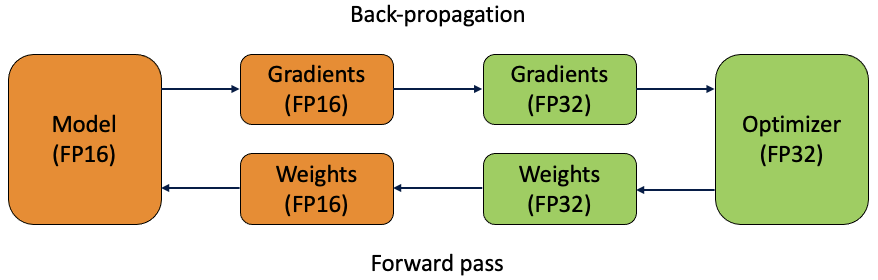
여기에서 가중치의 FP32 사본을 유지하는 이점을 볼 수 있습니다.학습률이 종종 작기 때문에 가중치 기울기를 곱하면 종종 작은 값이 될 수 있습니다.FP16의 경우 크기가 2 ^ (-24)보다 작은 숫자는 표현할 수 없기 때문에 0과 동일합니다 (FP16의 비정규 화 된 한계입니다).따라서 FP32에서 업데이트를 완료하면 이러한 업데이트 값을 유지할 수 있습니다.
FP16과 FP32를 모두 사용하기 때문에이 기술이 호출됩니다.혼합-정밀 교육.
손실 스케일링
혼합 정밀도 훈련은 대부분 정확도 유지 문제를 해결했지만 실험 결과 학습률을 곱하기 전에도 작은 기울기 값이 발생하는 경우가있었습니다.
NVIDIA 팀은 2 ^ -27 미만의 값이 주로 훈련과 관련이 없지만 보존하는 데 중요한 [2 ^ -27, 2 ^ -24) 범위의 값이 있지만 FP16 한계를 벗어난 값이 있음을 보여주었습니다.훈련 반복 동안 0으로 동일시합니다.정밀도 한계로 인해 기울기가 0과 같은이 문제를 언더 플로우라고합니다.
따라서 그들은 손실 스케일링을 제안하는데, 이는 순방향 패스가 완료된 후 역 전파 전에 손실 값에 스케일 팩터를 곱하는 프로세스입니다.그만큼연쇄 법칙모든 그라디언트가 FP16 범위 내에서 이동 한 동일한 요소에 의해 이후에 배율이 조정됨을 나타냅니다.
그래디언트가 계산되면 이전 섹션에서 설명한대로 FP32에서 마스터 가중치를 업데이트하는 데 사용되기 전에 동일한 배율로 나눌 수 있습니다.

NVIDIA “딥 러닝 성능”선적 서류 비치, 배율 인수 선택에 대해 설명합니다.이론적으로는 오버플로로 이어질만큼 충분히 크지 않는 한 큰 스케일링 계수를 선택하는 데 단점이 없습니다.
스케일링 계수를 곱한 기울기가 FP16의 최대 제한을 초과하면 오버플로가 발생합니다.이 경우 그래디언트가 무한이되고 NaN으로 설정됩니다.신경망 훈련의 초기 시대에 다음 메시지가 나타나는 것은 비교적 일반적입니다.
그라데이션 오버플로.스킵 단계, 손실 스케일러 0 손실 스케일 감소…
이 경우 무한 기울기를 사용하여 가중치 업데이트를 계산할 수없고 향후 반복을 위해 손실 척도가 감소하므로 단계를 건너 뜁니다.
자동 혼합 정밀도
2018 년에 NVIDIA는파이 토치전화꼭대기, 여기에는 AMP (자동 혼합 정밀도) 기능이 포함되어 있습니다.이것은 PyTorch에서 혼합 정밀도 훈련을 사용하기위한 간소화 된 솔루션을 제공했습니다.
단 몇 줄의 코드로 훈련을 FP32에서 GPU의 혼합 정밀도로 이동할 수 있습니다.이것은두 가지 주요 이점:
- 훈련 시간 단축— 훈련 시간은 모델 성능의 현저한 감소없이 1.5 배에서 5.5 배까지 감소 된 것으로 나타났습니다.
- 메모리 요구 사항 감소— 이것은 아키텍처 크기, 배치 크기 및 입력 데이터 크기와 같은 다른 모델 요소를 증가시키기 위해 메모리를 확보했습니다.
PyTorch 1.6부터 NVIDIA와 Facebook (PyTorch의 제작자)은이 기능을 핵심 PyTorch 코드로 옮겼습니다.torch.cuda.amp.이를 통해 버전 호환성 및 확장 빌드의 어려움과 같은 Apex 패키지를 둘러싼 몇 가지 문제점이 해결되었습니다.
이 기사에서는 AMP의 코드 구현에 대해 더 이상 설명하지 않지만 PyTorch에서 예제를 볼 수 있습니다.선적 서류 비치.
결론
부동 소수점 정밀도는 종종 간과되지만 딥 러닝 모델의 훈련에서 중요한 역할을합니다. 여기서 작은 기울기와 학습률이 증가하여 더 많은 비트를 정확하게 표현해야하는 기울기 업데이트를 생성합니다.
그러나 최첨단 딥 러닝 모델이 작업 성능 측면에서 경계를 확장함에 따라 아키텍처가 성장하고 정밀도가 훈련 시간, 메모리 요구 사항 및 사용 가능한 컴퓨팅과 균형을 이루어야합니다.
따라서 본질적으로 메모리 사용량을 절반으로 줄이면서 성능을 유지하는 혼합 정밀도 훈련의 능력은 딥 러닝의 중요한 발전입니다!
Understanding Mixed Precision Training
Understanding Mixed Precision Training
Mixed precision for training neural networks can reduce training time and memory requirements without affecting model performance
As deep learning methodologies have developed, it has been generally agreed that increasing the size of a neural network improves performance. However, this is at the detriment of memory and compute requirements, which also need to be increased to train the model.
This can be put into perspective by comparing the performance of Google’s pre-trained language model, BERT, at different architecture sizes. In the original paper, Google’s researchers reported an average GLUE score of 79.6 for BERT-Base and 82.1 for BERT-Large. This small increase of 2.5 came with an extra 230M parameters (110M vs. 340M)!
As a rough calculation, if each parameter is stored in single precision (more detail below), which is 32 bytes of information, then 230M parameters is equivalent to 0.92Gb in memory. This may not seem too large in and of itself, but consider that during each training iteration these parameters goes through a series of steps of matrix arithmetics, calculating further values, such as gradients. All these extra values can quickly become unmanageable.
In 2017, a group of researchers from NVIDIA released a paper detailing how to reduce the memory requirements of training neural networks, using a technique called Mixed Precision Training:
We introduce methodology for training deep neural networks using half-precision floating point numbers, without losing model accuracy or having to modify hyperparameters. This nearly halves memory requirements and, on recent GPUs, speeds up arithmetic.
In this article, we will explore mixed-precision training, understanding both how it fits into the standard algorithmic framework of deep learning and how it is able to reduce computational demand without affecting model performance.
Floating Point Precision
The technical standard used for representing floating-point numbers in binary formats is IEEE 754, established in 1985 by the Institute of Electrical and Electronics Engineering.
As set out in IEEE 754, there are various levels of floating-point precision, ranging from binary16 (half-precision) to binary256 (octuple-precision), where the number after “binary” equals the number of bits available for representing the floating-point value.
Unlike integer values, where the bits simply represent the binary form of the number, perhaps with a single bit reserved for the sign, floating-point values also need to consider an exponent. Therefore, the representation of these numbers in binary form is more nuanced and can significantly affect precision.
Historically, deep learning has used single-precision (binary32, or FP32) to represent parameters. In this format, one bit is reserved for the sign, 8 bits for the exponent (-126 to +127) and 23 bits for the digits. Half-precision, or FP16, on the other hand, reserves one bit for the sign, 5 bits for the exponent (-14 to +14) and 10 for the digits.
However, this comes at a cost. The smallest and largest positive, normal values for each are as follows:
As well as this, smaller denormalized numbers can be represented, where all the exponent bits are set to zero. For FP16, the absolute limit is 2^(-24) However, as denormalized numbers get smaller, the precision decreases.
We will not go into any further depth here to understand the quantitative limitations of different floating-point precision in this article, but the IEEE provides comprehensive documentation for further investigation.
Mixed Precision Training
During standard training of neural networks FP32 to represent model parameters at the cost of increased memory requirements. In mixed-precision training, FP16 is used instead to store the weights, activations and gradients during training iterations.
However, as we saw above this creates a problem, as the range of values that can be stored by FP16 is smaller than FP32, and precision decreases as number become very small. The result of this would be a decrease in the accuracy of the model, in line with the precision of the floating-point values calculated.
To combat this, a master copy of the weights is stored in FP32. This is converted into FP16 during part of each training iteration (one forward pass, back-propagation and weight update). At the end of the iteration, the weight gradients are used to update the master weights during the optimizer step.
Here, we can see the benefit of keeping the FP32 copy of the weights. As the learning rate is often small, when multiplied by the weight gradients they can often be tiny values. For FP16, any number with magnitude smaller than 2^(-24) will be equated to zero as it cannot be represented (this is the denormalized limit for FP16). Therefore, by completing the updates in FP32, these update values can be preserved.
The use of both FP16 and FP32 is the reason this technique is called mixed-precision training.
Loss Scaling
Although mixed-precision training solved, in the most part, the issue of preserving accuracy, experiments showed that there were cases where small gradient values occurred, even before being multiplied by the learning rate.
The NVIDIA team showed that, although values below 2^-27 were mainly irrelevant to training, there were values in the range [2^-27, 2^-24) which were important to preserve, but outside of the limit of FP16, equating them to zero during the training iteration. This problem, where gradients are equated to zero due to precision limits, is known as underflow.
Therefore, they suggest loss scaling, a process by which the loss value is multiplied by a scale factor after the forward pass is completed and before back-propagation. The chain rule dictates that all the gradients are subsequently scaled by the same factor, which moved them within the range of FP16.
Once the gradients have been calculated, they can then be divided by the same scale factor, before being used to update the master weights in FP32, as described in the previous section.
In the NVIDIA “Deep Learning Performance” documentation, the choice of scaling factor is discussed. In theory, there is no downside to choosing a large scaling factor, unless it is large enough to lead to overflow.
Overflow occurs when the gradients, multiplied by the scaling factor, exceed the maximum limit for FP16. When this occurs, the gradient becomes infinite and is set to NaN. It is relatively common to see the following message appear in the early epochs of neural network training:
Gradient overflow. Skipping step, loss scaler 0 reducing loss scale to…
In this case, the step is skipped, as the weight update cannot be calculated using an infinite gradient, and the loss scale is reduced for future iterations.
Automatic Mixed Precision
In 2018, NVIDIA released an extension for PyTorch called Apex, which contained AMP (Automatic Mixed Precision) capability. This provided a streamlined solution for using mixed-precision training in PyTorch.
In only a few lines of code, training could be moved from FP32 to mixed precision on the GPU. This had two key benefits:
- Reduced training time — training time was shown to be reduced by anywhere between 1.5x and 5.5x, with no significant reduction in model performance.
- Reduced memory requirements — this freed up memory to increase other model elements, such as architecture size, batch size and input data size.
As of PyTorch 1.6, NVIDIA and Facebook (the creators of PyTorch) moved this functionality into the core PyTorch code, as torch.cuda.amp. This fixed several pain points surrounding the Apex package, such as version compatibility and difficulties in building the extension.
Although this article will not go any further into the code implementation of AMP, examples can be seen in the PyTorch documentation.
Conclusion
Although floating-point precision is often overlooked, it plays a key role in the training of deep learning models, where small gradients and learning rates multiply to create gradient updates that require more bits to be precisely represented.
However, as state-of-the-art deep learning models push the boundaries in terms of task performance, architectures grow and precision has to be balanced against training time, memory requirements and available compute.
Therefore, the ability of mixed precision training to maintain performance whilst essentially halving the memory usage is a significant advance in deep learning!