
2021년 2월 3일 용인시 부동산 경매 데이터 분석
경기도 용인시 수지구 죽전로27번길 14-30, 604동 5층 504호 (죽전동,꽃메마을한라신영프로방스) [집합건물 철근콘크리트구조 148.864㎡]
| 항목 | 값 |
|---|---|
| 경매번호 | 2013타경51772 |
| 경매날짜 | 2021.02.17 |
| 법원 | 수원지방법원 |
| 담당 | 경매5계 |
| 감정평가금액 | 873,000,000 |
| 경매가 | 873,000,000(100%) |
| 유찰여부 | 유찰\t1회 |
<최근 1년 실거래가 정보>
– 총 거래 수: 34건
– 동일 평수 거래 수: 13건

최근 1년 동일 평수 거래건 보기
| 날짜 | 전용면적 | 층 | 가격 |
|---|---|---|---|
| 2021-01-04 | 148.864 | 7 | 89900 |
| 2020-12-02 | 148.864 | 5 | 94000 |
| 2020-10-13 | 148.864 | 18 | 82000 |
| 2020-10-26 | 148.864 | 22 | 84300 |
| 2020-07-20 | 148.864 | 22 | 86000 |
| 2020-07-29 | 148.864 | 10 | 82000 |
| 2020-07-04 | 148.864 | 13 | 79800 |
| 2020-06-16 | 148.864 | 8 | 75000 |
| 2020-06-16 | 148.864 | 19 | 79500 |
| 2020-06-04 | 148.864 | 21 | 75000 |
| 2020-05-18 | 148.864 | 15 | 75000 |
| 2020-02-10 | 148.864 | 16 | 75000 |
| 2020-02-19 | 148.864 | 3 | 70000 |
2021년 2월 2일 모바일 게임 매출 순위
| Rank | Game | Publisher |
|---|---|---|
| 1 | 리니지M | NCSOFT |
| 2 | 리니지2M | NCSOFT |
| 3 | 세븐나이츠2 | Netmarble |
| 4 | 그랑사가 | NPIXEL |
| 5 | Cookie Run: Kingdom | Devsisters Corporation |
| 6 | 기적의 검 | 4399 KOREA |
| 7 | R2M | Webzen Inc. |
| 8 | 블레이드&소울 레볼루션 | Netmarble |
| 9 | 라이즈 오브 킹덤즈 | LilithGames |
| 10 | 바람의나라: 연 | NEXON Company |
| 11 | A3: 스틸얼라이브 | Netmarble |
| 12 | V4 | NEXON Company |
| 13 | S.O.S:스테이트 오브 서바이벌 | KingsGroup Holdings |
| 14 | Genshin Impact | miHoYo Limited |
| 15 | 뮤 아크엔젤 | Webzen Inc. |
| 16 | 메이플스토리M | NEXON Company |
| 17 | 미르4 | Wemade Co., Ltd |
| 18 | FIFA ONLINE 4 M by EA SPORTS™ | NEXON Company |
| 19 | 찐삼국 | ICEBIRD GAMES |
| 20 | 리니지2 레볼루션 | Netmarble |
| 21 | 검은강호2: 이터널 소울 | 9SplayDeveloper |
| 22 | Lords Mobile: Kingdom Wars | IGG.COM |
| 23 | Brawl Stars | Supercell |
| 24 | KartRider Rush+ | NEXON Company |
| 25 | Cookie Run: OvenBreak – Endless Running Platformer | Devsisters Corporation |
| 26 | Roblox | Roblox Corporation |
| 27 | 가디언 테일즈 | Kakao Games Corp. |
| 28 | Age of Z Origins | Camel Games Limited |
| 29 | PUBG MOBILE | KRAFTON, Inc. |
| 30 | 블리치: 만해의 길 | DAMO NETWORK LIMITED |
| 31 | Empires & Puzzles: Epic Match 3 | Small Giant Games |
| 32 | AFK 아레나 | LilithGames |
| 33 | Gardenscapes | Playrix |
| 34 | 프린세스 커넥트! Re:Dive | Kakao Games Corp. |
| 35 | FIFA Mobile | NEXON Company |
| 36 | Summoners War | Com2uS |
| 37 | Homescapes | Playrix |
| 38 | 그랑삼국 | YOUZU(SINGAPORE)PTE.LTD. |
| 39 | Top War: Battle Game | Topwar Studio |
| 40 | Dungeon Knight: 3D Idle RPG | mobirix |
| 41 | 갑부: 장사의 시대 | BLANCOZONE NETWORK KOREA |
| 42 | Pmang Poker : Casino Royal | NEOWIZ corp |
| 43 | 라그나로크 오리진 | GRAVITY Co., Ltd. |
| 44 | 한게임 포커 | NHN BIGFOOT |
| 45 | Epic Seven | Smilegate Megaport |
| 46 | 검은사막 모바일 | PEARL ABYSS |
| 47 | Pokémon GO | Niantic, Inc. |
| 48 | Destiny Child : Defense War | THUMBAGE |
| 49 | 컴투스프로야구2021 | Com2uS |
| 50 | 마구마구 2020 | Netmarble |
Analyzing Erasmus Study Exchanges with Pandas -번역
판다와 에라스무스 연구 교환 분석
Erasmus 프로그램 2011–12에서 발생한 20 만 개의 연구 교환으로 데이터 세트를 분석 한 결과
1987 년 이래, Erasmus 프로그램은 매년 수십만 명의 유럽 학생들에게 한 학기 또는 1 년을 다른 유럽 국가에서 해외로 보낼 수있는 기회를 제공하여 학생들에게 쉬운 교환 과정과 경제적 지원을 제공합니다.유럽의 다양한 사람, 언어 및 문화에 대한 마음과 마음을 열어주는 정말 귀중한 경험입니다.
Aust 비엔나에서 에라스무스 교환을 했어요아르 자형ia, 그리고 그것은 또한 잊을 수없는 경험이었습니다.데이터 분석에 대한 프로젝트를 수행해야하는 과정이있었습니다.힐케 반 뮈 르스그리고 나는 분석을하기로 결정했다2011-12 학년도 에라스무스 교환 데이터, 사용 가능유럽 연합 개방형 데이터 포털.1 년 후 오늘 저는이 프로젝트를 여러분과 공유하고 있습니다.
설정
이 과제에서 우리가 가진 주요 요구 사항은JupyterLab작업 환경으로파이썬프로그래밍 언어로판다데이터 처리 라이브러리로.또한 우리는Matplotlib일부 그래프를 그릴뿐만 아니라Scipy과Numpy일부 작업을 수행합니다.
데이터 이해
그만큼데이터 세트,에서 다운로드유럽 연합 개방형 데이터 포털, CSV 파일로, 각 행은 한 학생을 나타내고 열은 그녀가오고가는 국가 및 대학, 학업 분야, 교환 기간 등 교환에 대한 정보를 제공합니다.

칼럼이 많고이 프로젝트에 쓸모없는 칼럼이 많으므로 지금 각각을 설명하는 대신 필요할 때마다 그 의미를 설명하겠습니다.또 다른 중요한 사실은이 데이터 세트가 연구 교환뿐만 아니라 인턴십과 같은 다른 유형의 에라스무스 배치에 대한 정보를 제공한다는 것입니다.이 프로젝트는 연구 교류에만 집중할 것이기 때문에, 곧 보게 될 다른 프로젝트는 삭제 될 것입니다.
데이터 다운로드 및 정리
그러니 일하러 가자!먼저 JupyterLab에서 새 노트북을 만들고 필요한 기본 라이브러리를 가져오고 플로팅 스타일을 설정하는 것으로 시작하겠습니다.
그런 다음 유럽 연합 데이터 포털 서버에서 데이터 세트를 다운로드하고이를 Pandas DataFrame으로 변환해야합니다.
마지막으로,이 데이터 세트는 학습 및 인턴십 교환을 모두 다루며 학습 교환에만 집중하기를 원하므로 게재 위치에 해당하는 행과 열을 제거합니다.
단일 변수 분석
연령,받은 보조금 및 크레딧 수
이제 데이터를 분석 할 준비가되었으므로 학생의 나이, 학생이받는 보조금 또는 ECTS (크레딧) 수와 같은 일부 단일 변수에 대한 최소, 최대, 평균 및 표준 편차를 계산하여 시작하겠습니다.연구.데이터를 더 잘 이해하기 위해 히스토그램으로 표시합니다.
예를 들어 학생의 연령에 대한 통계 지표를 얻는 방법을 살펴 보겠습니다 (열나이) :
2011-12 세의 막내 에라스무스 학생은 겨우 17 세였습니다. 놀랍습니다!하지만 가장 놀라운 것은 가장 나이가 83 세라는 것이 믿기지 않습니다.우리는 너무 충격을 받아이 사람에 대한 더 많은 정보를 위해 데이터 셋을 검색했고, 갑자기이 교환 프로그램에 참여하기로 결정한 것은 한 명뿐 아니라 두 명의 영국 신사였습니다.그럼에도 불구하고 평균 연령은 22 세입니다.
총계 (연구자) 및 월간 (STUDYGRANT / LENGTHSTUDYPERIOD)받은 보조금 및 크레딧 수 (TOTALECTSCREDITS) – 전체 노트북에서 코드를 찾을 수 있습니다 –.
성별 비율
남녀 비율을 결정하는 것도 매우 흥미로울 수 있습니다.이것은 얻을 수 있습니다성별DataFrame의 열과‘에프’(여성) 및‘미디엄’(남성) :
쉽죠?남성의 39.41 %에 비해 학생의 60.59 %가 여성 인 것 같습니다.그러나이 비율은 나중에 살펴 보 겠지만 대상 대학마다 크게 다릅니다.
대학 보내기 및 받기
더 많은 학생들을 해외로 보내는 유럽 대학이 무엇인지 궁금하십니까?그런 다음‘홈 인스 티 튜션’데이터 프레임에서 고유 한 값과 빈도를value_counts ()메서드를 사용하고 막대 그래프로 플로팅합니다.

받는 기관의 상위 10 개를 얻으려면‘홈 인스 티 튜션’와‘HOSTINSTITUTION’및 voilà!10 대 발송 기관 중 8 개 기관이 수신 기관 상위 10 개 기관에 속한다는 것은 말할 필요도 없습니다.
언어
영어는 보편적 언어로 간주되지만 유럽 학생들이 교환을 위해 해외에 갈 때 셰익스피어 언어로 과정을 수강한다는 의미는 아닙니다.데이터 세트의 각 학생에 대해LANGUAGETAUGHT열은 코스를받은 언어를 제공하므로 코스에서 가장 많이 사용되는 10 가지 언어를 플로팅 해 보겠습니다.
예상대로 영어가 10 만 3 천명으로 가장 인기가 많았고, 스페인어가 2 만 7 천명으로 거의 4 배나 낮았습니다.

그렇다면 이것은 영국과 아일랜드에서 에라스무스 학생들이 영어 코스를 수강하는 비율이 스페인에서 스페인어, 프랑스에서 프랑스어로 수강하는 것보다 훨씬 높다는 것을 의미합니까?찾아 보자!

전혀!영국의 에라스무스 학생의 91.9 %가 영어로 배우고 있습니다 (영국에서도 영어의 전능함에도 불구하고 외국어 코스가 있음), 아일랜드의 86.8 %가 그 뒤를이었습니다.3 위는 스페인 에라스무스 학생의 84.5 %가 스페인어로 수강했으며 4 위는 프랑스 학생의 81.1 %가 프랑스어로 이수했습니다.1 위와 5 위 (영국과 이탈리아)의 차이는 14 %에 불과합니다.
주제 영역
또 다른 필수 질문은 에라스무스 학생들이 가장 인기있는 과목과 덜 인기있는 과목입니다.에 따르면유네스코의 ISCED 분류, 9 개의 연구 영역이 있습니다.교육, 인문학 & amp;예술, 사회 과학 & amp;비즈니스 & amp;법률, 과학, 공학 및제조 & amp;건설, 농업, 건강 및복지 및 서비스.데이터 세트의 각 행에 대해 학생의 주제 영역을 나타내는 숫자가 열에 있습니다.대상 지역.그러나 해당 필드에서는 첫 번째 숫자 만 필요하므로 코드에주의하십시오.람다함수:
8 만 명 이상의 학생들이있는 가장 인기있는 학습 영역은사회 과학, 비즈니스 및 법률.은메달과 동메달은인문학 & amp;기예과엔지니어링, 제조 및구성, 각각 44.7k 및 30.8k 학생.

여러 변수 분석
대학 수혜에 따른 성별 비율
유럽에“여대”나“남학생”이 있는지 생각해 본 적이 있습니까?글쎄, 우리는 남학생이나 여학생 만받는 기관이 많다는 사실을 알고 깜짝 놀랐습니다.우리는 신입 여학생의 비율로 상위 30 대 대학을 쉽게 순위를 매길 수 있으며, 다른 학생은 신입생을위한 상위 30 대 대학으로 쉽게 순위를 매길 수 있습니다.
놀랍게도 두 순위 모두에서 남성 또는 여성의 비율은 100 %입니다.처음 123 개 대학을 인쇄하지 않는 한 남성의 100 %보다 낮은 비율이 표시되지 않으며 처음 256 개 기관을 나열하지 않는 한 여성도 마찬가지입니다.
대학 수강 기준 평균 연령
가장 나이가 많은 대학과 가장 어린 대학이 어디인지 궁금하십니까?
최연소 순위에서는 18 (IES Poblenou, Barcelona – 사실 대학이 아니라 기술 대학 센터 –)에서 상위 10 위의 19.5 년까지 차이가 거의 없지만 가장 오래된 순위에서는 차이가 다음과 같습니다.더 높은 : 45 년Hochschule 21독일에서 10 위는Lyceé Albert Camus, 프랑스에서 입학하는 학생들의 평균 연령은 32 세입니다.
국가 별 신입생 비율
제가 태어난 나라 인 스페인은 유학을가는 유럽 학생들이 가장 원하는 곳 중 하나입니다.그럼에도 불구하고 많은 스페인 학생들도 저처럼 에라스무스를 다니기 때문에 비율이 상당히 균형을 이룹니다.그러나 해외로 많은 학생을 파견하지만 거의받지 못하는 국가가 있으며 그 반대의 경우도 마찬가지입니다.막대 그래프를 통해 각 국가의 송수신 비율을 쉽게 확인할 수 있습니다.
변수 간의 상관 관계 분석
본국 및 호스트 국가
본국 및 목적지 국가는 숫자가 아닌 범주 형 변수이므로 상관 지수를 계산하는 것은 간단하지 않습니다.이러한 이유로 우리는 히트 맵과 같이 더 시각적 인 것을 선택했습니다.

위의 히트 맵에서 각 행은 모국을 나타내고 각 열은 목적지를 나타냅니다.결과는 각 국가에 대해 정규화됩니다. 즉, 색상은 각 목적지 (열)를 선택한 각 국가 (행)의 학생 비율을 나타냅니다.이 차트에서 보면이 변수 쌍의 엔트로피가 매우 낮은 것 같습니다. 즉, 특정 국가의 경우 선호하는 목적지가 어디인지 예측할 수 있음을 의미합니다.한 국가에 대해 확인해 보겠습니다.

본국과 목적지 국가간에 상관 관계가없는 경우, 각 본국에 대해 각 목적지 국가는 2.86 %의 학생을 받게됩니다.그러나 위의 히트 맵과 원형 차트에서 모두 그렇게 보이지 않습니다.예를 들어, 원형 차트에서 스페인 학생들이 이탈리아 (21.3 %), 프랑스 (12.4 %), 독일 (11.1 %), 영국 (9.4 %), 포르투갈 (6.8 %) 및 폴란드 (6.6 %).
목적지 및 주제 영역
유럽에는 매우 명망있는 대학이 있지만 모든 지식 영역에서 탁월한 대학을 찾기는 매우 어렵습니다.그렇기 때문에 각 과목에 대해 다른 기관보다 일부 기관에 대한 선호도가 있는지 확인하는 것이 흥미로울 것입니다.다시 범주 형 변수를 다루고 있으므로 이전과 동일한 기법을 적용 해 보겠습니다.
학과목과 목표 대학의 상관 관계가 0이면 각 학과목에 대해 각 목표 대학은 학생의 0.04 %를 받게된다.그러나 대부분의 교과 영역에서 더 많은 학생을받는 기관은 1 %에서 3.7 % 사이로 두 변수 간의 엔트로피가 높지 않음을 보여줍니다.그러나 이런 의미에서 우리는 나머지를 강조하는 대학을 찾을 수 없었습니다.“일반”범주에 대한 비율은 놀랍고 3 개 기관 만이 학생의 거의 50 %를받습니다.
가정 및 호스트 국가 및 월별 보조금
2019 년에 에라스무스 교환을 위해 서류 작업을 할 때 스페인 정부가 생활비에 따라 세 그룹의 목적지 국가를 설정하여 각기 다른 월별 보조금을 제공 한 것을 기억합니다.제가 그곳에 갔을 때 다른 유럽 국가에서 온 친구들이 저보다 더 많거나 적은 돈을받는 것을보고 놀랐습니다.그렇다면 월별 보조금은 무엇에 의존합니까? 당신이 가고자하는 국가 또는 당신이 오는 국가?찾아 보자!

두 플롯을 비교하고 엄청난 양의 이상 값을 제거하면 학생들이받는 금액에서 본국이 목적지 국가보다 더 결정적인 요소임을 알 수 있습니다.첫 번째 그림에서 각 목적지 국가의 월별 보조금 평균은 매우 동질적인 것으로 보이며 대부분의 경우 평균값의 50 %에서 150 %까지 분산이 매우 높습니다.두 번째 플롯은 분산이 매우 낮고 평균 보조금은 매우 이질적입니다.따라서이 분석을하기 전에 예상했듯이 월별 보조금은 주로 귀하가 출신 국가에 달려 있습니다.
글이 너무 길지 않았 으면 좋겠습니다.사실,이 글에서는 너무 길지 않기 위해 우리가 만든 몇 가지 통찰력을 건너 뛰었습니다. 관심이 있다면 여기에완전한 노트북.나는 또한 다시 한 번 외침을하고 싶다힐케 반 뮈 르스이 프로젝트에 투입된 작업을 위해.물론 질문이나 제안이 있으시면 댓글로 알려주세요.
참고
- JupyterLab :https://jupyter.org/install
- Pandas DataFrame :https://pandas.pydata.org/pandas-docs/stable/reference/api/pandas.DataFrame.html
- Matplotlib :https://matplotlib.org/api/
- Erasmus 2011–12 데이터 세트 :https://data.europa.eu/euodp/en/data/dataset/erasmus-mobility-statistics-2011-12
- GitHub의 Jupyter 노트북 :https://github.com/gbarreiro/erasmus-data-analysis/blob/main/Erasmus.ipynb
Analyzing Erasmus Study Exchanges with Pandas
Analyzing Erasmus Study Exchanges with Pandas
The results of analyzing a dataset with the 200k study exchanges that took place in the Erasmus program 2011–12
Since 1987, the Erasmus program gives hundreds of thousands of European students every year the opportunity of spending a semester or a year abroad, in another European country, offering them an easy exchange process, as well as economic support. It’s a truly valuable experience, which opens their minds and hearts to the diverse people, languages, and cultures of Europe.
I did my Erasmus exchange in Vienna, Austria, and it was also an unforgettable experience. I had a course there where we had to do a project on data analysis, and Hilke van Meurs and I decided to do an analysis of the Erasmus exchange data for the academic year 2011–12, available in the European Union Open Data Portal. Today, one year later, I’m sharing with you this project.
Setup
The main requirements we had in this assignment were to use JupyterLab as the working environment, Python as programming language, and Pandas as the data processing library. In addition, we had to use Matplotlib for plotting some graphs, as well as Scipy and Numpy for performing some operations.
Understanding the Data
The dataset, downloaded from the European Union Open Data Portal, is a CSV file where each row represents a single student, and the columns give information about her exchange, like country and university she’s coming from and going to, area of study, exchange length…
There are a lot of columns, and many of them useless for this project, so instead describing each of them now, I’ll be explaining its meaning whenever we need to use them. Another important fact is that this dataset offers information not only about the study exchanges, but also other type of Erasmus placements, like internships. Since this project will only focus on study exchanges, the others will be dropped, as we will shortly see.
Downloading and Cleaning the Data
So let’s get to work! First of all, let’s start by creating a new notebook in JupyterLab, importing some basic libraries we’ll need, and setting up the plotting styles:
Then we have to download the dataset from the European Union Data Portal servers and convert it to a Pandas DataFrame:
Finally, since this dataset covers both studying and internships exchanges and we want to focus only in the study exchanges, we’ll remove the rows and columns corresponding to placements:
Analyzing Single-Variables
Age, received grant, and number of credits
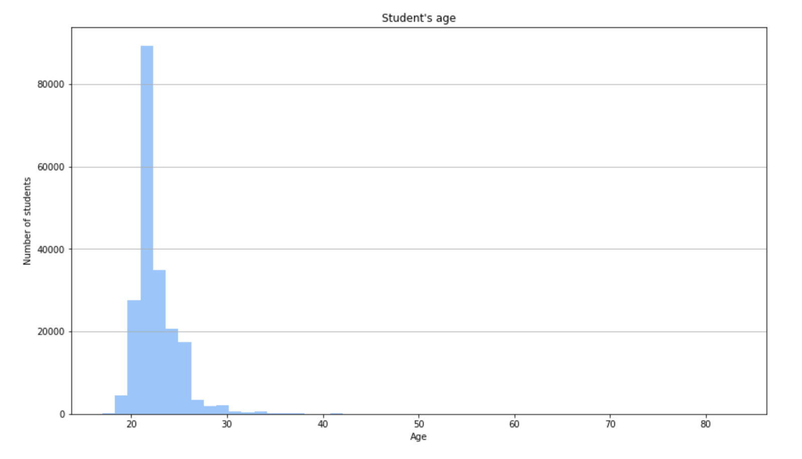
Now that our data is ready to be analyzed, let’s begin by calculating the minimum, maximum, average, and standard deviation for some single variables, like the age of the students, the grant they receive, or the number of ECTS (credits) they study. For better understanding that data, we’ll also plot it in histograms.
For example, let’s see how to get those statistical indicators for the student’s age (column AGE):
The youngest Erasmus student in the 2011–12 year was only 17 years old, amazing! But what is most surprising is that the oldest was 83 years old, that’s unbelievable. We were so shocked that we searched in the dataset for more information about this person, and out of the blue, it was not only one, but two British gentlemen who decided to go on this exchange program. Nevertheless, the average age is 22 years.
The same would apply for the total (STUDYGRANT) and monthly (STUDYGRANT/LENGTHSTUDYPERIOD) received grant and number of credits (TOTALECTSCREDITS) –you can find the code in the complete notebook–.
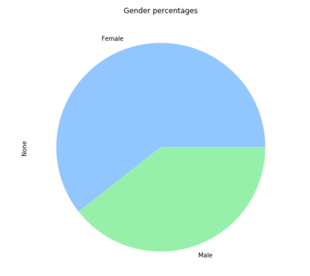
Gender percentage
It can also be very interesting to determine the male-female percentage. This can be done by getting the GENDER column from the DataFrame and counting the number of occurrences of ‘F’ (female) and ‘M’ (male):
Easy, right? It looks like 60.59% of the students were women, against a 39.41% of men. However, I this ratio varies enormously across different destination universities, as we’ll see later.
Sending and receiving universities
Are you curious about which are the European universities that send more students abroad? Then, just get the column ‘HOMEINSTITUTION’ from the DataFrame, calculate its unique values and its frequency with the value_counts() method, and plot it in a bar graph:
If you want to get the top 10 for receiving institutions, just replace ‘HOMEINSTITUTION’ with ‘HOSTINSTITUTION’ and voilà! It goes without saying that 8 out of the 10 top sending institutions are also in the top 10 receiving ones.
Languages
English is considered to be the universal language, but that doesn’t mean that European students take their courses in the Shakespeare language when they go abroad for an exchange. For each student in the dataset, the LANGUAGETAUGHT column give us the language in which they received their courses, so let’s plot the ten most popular languages for the courses:
As we would expect, English is by far the most popular, with 103k students, followed by Spanish, with 27k, almost 4 times lower.
So, does this mean that in the UK and Ireland the percentage of Erasmus students taking their courses in English is much higher than in Spain taking them in Spanish, French in France and so on? Let’s find it out!
Not at all! 91.9% of the Erasmus students in the UK are learning in English (so even in the UK there are courses in foreign languages, despite the omnipotence of English language), followed by a 86.8% in Ireland. In third place, a 84.5% of the Erasmus students in Spain took their courses in Spanish, and in fourth place, 81.1% of the students in France took them in French. The difference between the 1st and 5th country (UK and Italy) is just of a 14%.
Subject areas
Another essential question is which are the most and less popular subject areas of the Erasmus students. According to the UNESCO’S ISCED classification, there are nine study areas: Education, Humanities & Arts, Social sciences & business & law, Science, Engineering & manufacturing & construction, Agriculture, Health & Welfare, and Services. For each row of our dataset, a number representing the subject area of the student is available at the column SUBJECTAREA. However, from that field we only need the first digit, so pay attention to the code, since it has a tricky lambda function:
With more than 80k students, the most popular study area by far is Social Sciences, business and law. The silver and bronze medals go to Humanities & Arts and Engineering, Manufacturing & Construction, with 44.7k and 30.8k students respectively.
Analyzing Multiple Variables
Gender proportion by receiving university
Have you ever thought if there is a “girls university” or “boys university” in Europe? Well, we were quite surprised to know that there are many institutions that only received male or female students, did you know it? We can easily make a ranking of the top 30 universities in percentage of incoming female students and another with the top 30 for incoming men.
Surprisingly, in both rankings, the percentage of men or women is 100%. You won’t see a ratio lower than 100% of men unless you print the first 123 universities, neither for women unless you list the first 256 institutions.
Average age by receiving university
Wondering which are the universities that receive the oldest students, and which ones the youngest?
While in the youngest ranking the difference is very little, ranging from 18 (IES Poblenou, Barcelona –in fact, it’s not an university, but a technical college center–) to 19.5 years in the top 10, in the oldest ranking the difference is higher: 45 years for Hochschule 21 in Germany, while the 10th place is for the Lyceé Albert Camus, in France, with its incoming students having an average age of 32 years.
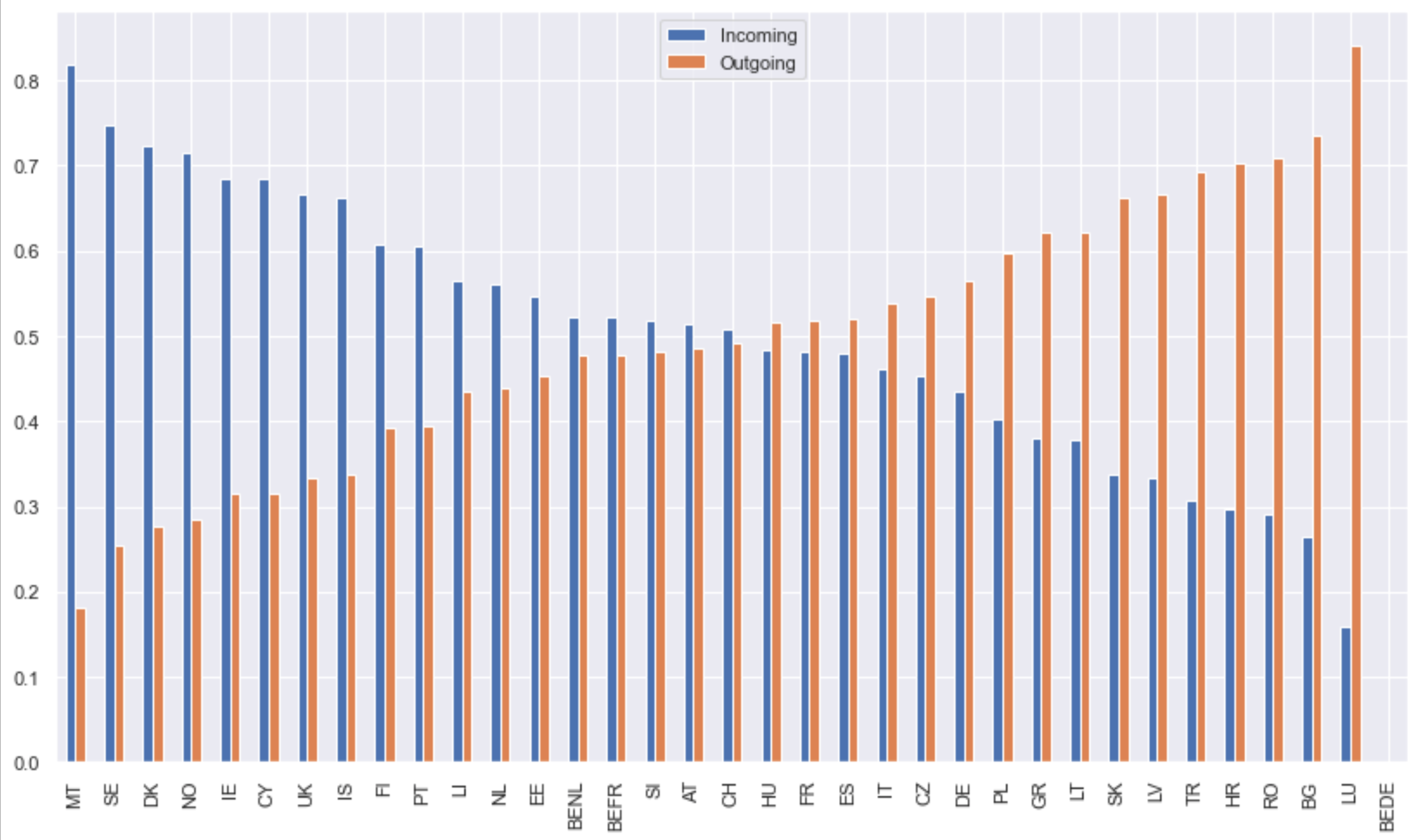
Ratio of incoming and outgoing students for each country
The country where I was born, Spain, it’s one of the most desired destinations for European students going abroad. Nevertheless, a lot of Spanish students go on an Erasmus too, like I did, so the proportion is quite balanced. However, there are countries that send a lot of students abroad, but barely receive any, and vice versa. With a bar plot, we can easily see the sending/receiving ratio for each country.
Analyzing Correlations Between Variables
Home and host country
The home and destination countries are categorical variables, not numeric, so calculating a correlation index wouldn’t be straightforward. For this reason, we opted for something more visual, like a heatmap.
In the heatmap above, each row represents a home country and each column a destination. The results are normalized for each home country, meaning that the colors represent the percentage of students from each country (rows) that chose each of the destinations (columns). From that chart, it looks like the entropy of this pair of variables is quite low, meaning that for a specific home country, it’s quite predictable which will be the preferred destinations. Let’s check it for one country:
If there were no correlation between the home and destination countries, for each home country, each destination country would receive 2.86% of the students. However, both in the heatmap and the pie chart above, it does not look like so. For instance, in the pie chart we can see how Spanish students have a huge preference for Italy (21.3%), France (12.4%), Germany (11.1%), UK (9.4%), Portugal (6.8%) and Poland (6.6%).
Destination and subject area
There are very prestigious universities around Europe, but it’s very difficult to find one that excels in every knowledge area. For that reason, it would be interesting to find out if for each subject area, there is a preference towards some institutions over others. Since we’re dealing again with categorical variables, let’s apply the same technique as before.
If the correlation between the subject area and the destination university were null, for each subject area, each destination university would receive 0.04% of the students. However, for most of the subject areas, the institution receiving more students has between a 1% and 3.7%, showing that the entropy between those two variables is not high. However, in this sense, we couldn’t find any university highlighting over the rest. The percentages for the “General” category are remarkable, with only three institutions receiving almost the 50% of the students.
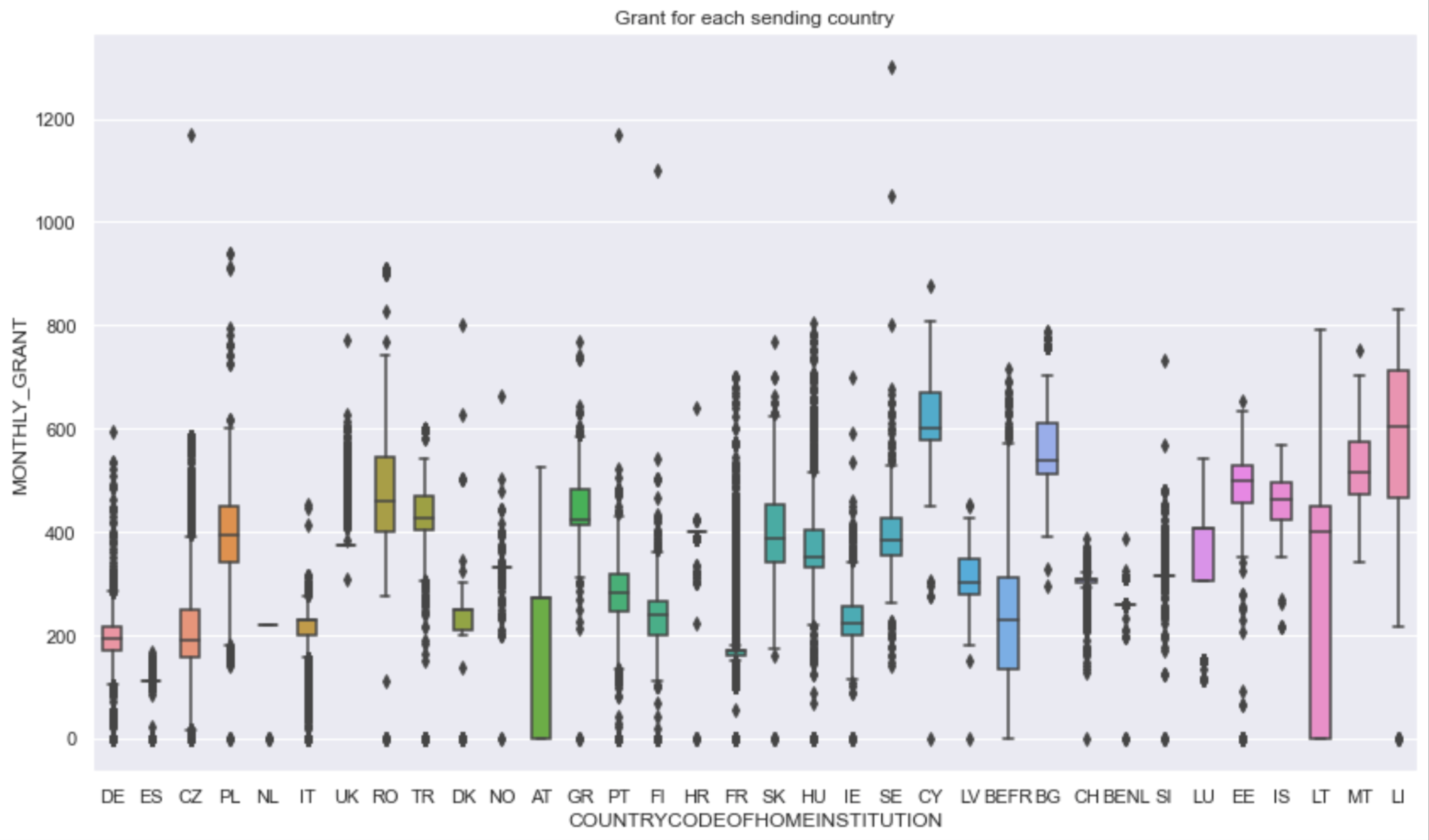
Home and host country and monthly grant
When I was doing the paperwork for my Erasmus exchange in 2019, I remember that the Spanish government set three groups of destination countries according the cost of life, giving a different monthly grant for each of them. Once I was there, I was surprised to see how some friends coming from other European countries received more or less money than I did. Then, what does the monthly grant depend on: the country you’re going to, or the one you’re coming from? Let’s find it out!
Comparing the two plots and obviating the enormous amount of outliers, it’s evident that the home country is a more deterministic factor than the destination country in the amount of money received by the students. In the first plot, it looks like the average of the monthly grant for each destination country is quite homogenous, and for most of them, the variance is very high, ranging from a 50% to a 150% of the average value, while in the second plot, the variance is really low, and the average grants are very heterogenous. Therefore, as I supposed before doing this analysis, the monthly grant depends mostly in the country you come from.
I hope that the post wasn’t too long for you. In fact, in this post I skipped some insights we made, to not make it too long, so if you’re interested, here you have the complete notebook. I would also like to give a shout-out again to Hilke van Meurs for the work put into this project. And of course, if you have any question or suggestion, please let me know in the comments.
Reference
- JupyterLab: https://jupyter.org/install
- Pandas DataFrame: https://pandas.pydata.org/pandas-docs/stable/reference/api/pandas.DataFrame.html
- Matplotlib: https://matplotlib.org/api/
- Erasmus 2011–12 Datasets: https://data.europa.eu/euodp/en/data/dataset/erasmus-mobility-statistics-2011-12
- Jupyter Notebook in GitHub: https://github.com/gbarreiro/erasmus-data-analysis/blob/main/Erasmus.ipynb
2021년 2월 1일 모바일 게임 매출 순위
| Rank | Game | Publisher |
|---|---|---|
| 1 | 리니지M | NCSOFT |
| 2 | 리니지2M | NCSOFT |
| 3 | 세븐나이츠2 | Netmarble |
| 4 | 그랑사가 | NPIXEL |
| 5 | Cookie Run: Kingdom | Devsisters Corporation |
| 6 | 기적의 검 | 4399 KOREA |
| 7 | 블레이드&소울 레볼루션 | Netmarble |
| 8 | 라이즈 오브 킹덤즈 | LilithGames |
| 9 | R2M | Webzen Inc. |
| 10 | 바람의나라: 연 | NEXON Company |
| 11 | FIFA ONLINE 4 M by EA SPORTS™ | NEXON Company |
| 12 | S.O.S:스테이트 오브 서바이벌 | KingsGroup Holdings |
| 13 | V4 | NEXON Company |
| 14 | 메이플스토리M | NEXON Company |
| 15 | A3: 스틸얼라이브 | Netmarble |
| 16 | Genshin Impact | miHoYo Limited |
| 17 | 뮤 아크엔젤 | Webzen Inc. |
| 18 | 미르4 | Wemade Co., Ltd |
| 19 | 리니지2 레볼루션 | Netmarble |
| 20 | 찐삼국 | ICEBIRD GAMES |
| 21 | 검은강호2: 이터널 소울 | 9SplayDeveloper |
| 22 | Lords Mobile: Kingdom Wars | IGG.COM |
| 23 | KartRider Rush+ | NEXON Company |
| 24 | Roblox | Roblox Corporation |
| 25 | Cookie Run: OvenBreak – Endless Running Platformer | Devsisters Corporation |
| 26 | Brawl Stars | Supercell |
| 27 | 블리치: 만해의 길 | DAMO NETWORK LIMITED |
| 28 | 가디언 테일즈 | Kakao Games Corp. |
| 29 | Age of Z Origins | Camel Games Limited |
| 30 | PUBG MOBILE | KRAFTON, Inc. |
| 31 | AFK 아레나 | LilithGames |
| 32 | Empires & Puzzles: Epic Match 3 | Small Giant Games |
| 33 | Gardenscapes | Playrix |
| 34 | 그랑삼국 | YOUZU(SINGAPORE)PTE.LTD. |
| 35 | FIFA Mobile | NEXON Company |
| 36 | Summoners War | Com2uS |
| 37 | Homescapes | Playrix |
| 38 | Top War: Battle Game | Topwar Studio |
| 39 | 갑부: 장사의 시대 | BLANCOZONE NETWORK KOREA |
| 40 | 프린세스 커넥트! Re:Dive | Kakao Games Corp. |
| 41 | Pmang Poker : Casino Royal | NEOWIZ corp |
| 42 | 검은사막 모바일 | PEARL ABYSS |
| 43 | 라그나로크 오리진 | GRAVITY Co., Ltd. |
| 44 | 한게임 포커 | NHN BIGFOOT |
| 45 | Pokémon GO | Niantic, Inc. |
| 46 | Dungeon Knight: 3D Idle RPG | mobirix |
| 47 | Epic Seven | Smilegate Megaport |
| 48 | 붕괴3rd | miHoYo Limited |
| 49 | Destiny Child : Defense War | THUMBAGE |
| 50 | 컴투스프로야구2021 | Com2uS |