
Analyzing Erasmus Study Exchanges with Pandas
The results of analyzing a dataset with the 200k study exchanges that took place in the Erasmus program 2011–12
Since 1987, the Erasmus program gives hundreds of thousands of European students every year the opportunity of spending a semester or a year abroad, in another European country, offering them an easy exchange process, as well as economic support. It’s a truly valuable experience, which opens their minds and hearts to the diverse people, languages, and cultures of Europe.
I did my Erasmus exchange in Vienna, Austria, and it was also an unforgettable experience. I had a course there where we had to do a project on data analysis, and Hilke van Meurs and I decided to do an analysis of the Erasmus exchange data for the academic year 2011–12, available in the European Union Open Data Portal. Today, one year later, I’m sharing with you this project.
Setup
The main requirements we had in this assignment were to use JupyterLab as the working environment, Python as programming language, and Pandas as the data processing library. In addition, we had to use Matplotlib for plotting some graphs, as well as Scipy and Numpy for performing some operations.
Understanding the Data
The dataset, downloaded from the European Union Open Data Portal, is a CSV file where each row represents a single student, and the columns give information about her exchange, like country and university she’s coming from and going to, area of study, exchange length…

There are a lot of columns, and many of them useless for this project, so instead describing each of them now, I’ll be explaining its meaning whenever we need to use them. Another important fact is that this dataset offers information not only about the study exchanges, but also other type of Erasmus placements, like internships. Since this project will only focus on study exchanges, the others will be dropped, as we will shortly see.
Downloading and Cleaning the Data
So let’s get to work! First of all, let’s start by creating a new notebook in JupyterLab, importing some basic libraries we’ll need, and setting up the plotting styles:
Then we have to download the dataset from the European Union Data Portal servers and convert it to a Pandas DataFrame:
Finally, since this dataset covers both studying and internships exchanges and we want to focus only in the study exchanges, we’ll remove the rows and columns corresponding to placements:
Analyzing Single-Variables
Age, received grant, and number of credits
Now that our data is ready to be analyzed, let’s begin by calculating the minimum, maximum, average, and standard deviation for some single variables, like the age of the students, the grant they receive, or the number of ECTS (credits) they study. For better understanding that data, we’ll also plot it in histograms.
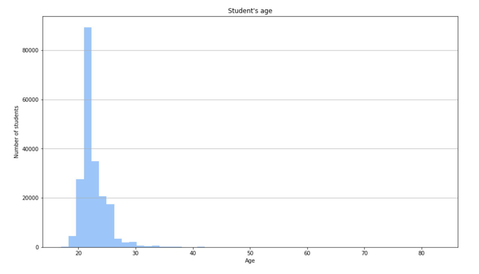
For example, let’s see how to get those statistical indicators for the student’s age (column AGE):
The youngest Erasmus student in the 2011–12 year was only 17 years old, amazing! But what is most surprising is that the oldest was 83 years old, that’s unbelievable. We were so shocked that we searched in the dataset for more information about this person, and out of the blue, it was not only one, but two British gentlemen who decided to go on this exchange program. Nevertheless, the average age is 22 years.
The same would apply for the total (STUDYGRANT) and monthly (STUDYGRANT/LENGTHSTUDYPERIOD) received grant and number of credits (TOTALECTSCREDITS) –you can find the code in the complete notebook–.
Gender percentage
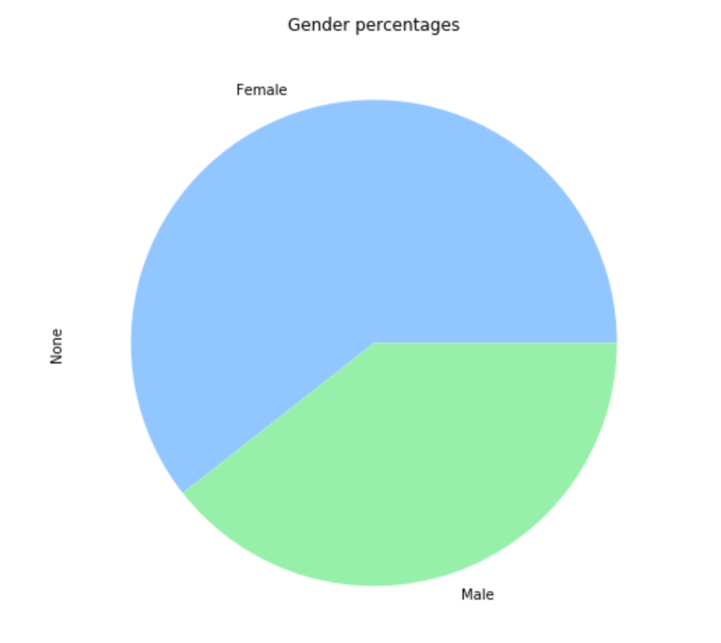
It can also be very interesting to determine the male-female percentage. This can be done by getting the GENDER column from the DataFrame and counting the number of occurrences of ‘F’ (female) and ‘M’ (male):
Easy, right? It looks like 60.59% of the students were women, against a 39.41% of men. However, I this ratio varies enormously across different destination universities, as we’ll see later.
Sending and receiving universities
Are you curious about which are the European universities that send more students abroad? Then, just get the column ‘HOMEINSTITUTION’ from the DataFrame, calculate its unique values and its frequency with the value_counts() method, and plot it in a bar graph:

If you want to get the top 10 for receiving institutions, just replace ‘HOMEINSTITUTION’ with ‘HOSTINSTITUTION’ and voilà! It goes without saying that 8 out of the 10 top sending institutions are also in the top 10 receiving ones.
Languages
English is considered to be the universal language, but that doesn’t mean that European students take their courses in the Shakespeare language when they go abroad for an exchange. For each student in the dataset, the LANGUAGETAUGHT column give us the language in which they received their courses, so let’s plot the ten most popular languages for the courses:
As we would expect, English is by far the most popular, with 103k students, followed by Spanish, with 27k, almost 4 times lower.

So, does this mean that in the UK and Ireland the percentage of Erasmus students taking their courses in English is much higher than in Spain taking them in Spanish, French in France and so on? Let’s find it out!

Not at all! 91.9% of the Erasmus students in the UK are learning in English (so even in the UK there are courses in foreign languages, despite the omnipotence of English language), followed by a 86.8% in Ireland. In third place, a 84.5% of the Erasmus students in Spain took their courses in Spanish, and in fourth place, 81.1% of the students in France took them in French. The difference between the 1st and 5th country (UK and Italy) is just of a 14%.
Subject areas
Another essential question is which are the most and less popular subject areas of the Erasmus students. According to the UNESCO’S ISCED classification, there are nine study areas: Education, Humanities & Arts, Social sciences & business & law, Science, Engineering & manufacturing & construction, Agriculture, Health & Welfare, and Services. For each row of our dataset, a number representing the subject area of the student is available at the column SUBJECTAREA. However, from that field we only need the first digit, so pay attention to the code, since it has a tricky lambda function:
With more than 80k students, the most popular study area by far is Social Sciences, business and law. The silver and bronze medals go to Humanities & Arts and Engineering, Manufacturing & Construction, with 44.7k and 30.8k students respectively.

Analyzing Multiple Variables
Gender proportion by receiving university
Have you ever thought if there is a “girls university” or “boys university” in Europe? Well, we were quite surprised to know that there are many institutions that only received male or female students, did you know it? We can easily make a ranking of the top 30 universities in percentage of incoming female students and another with the top 30 for incoming men.
Surprisingly, in both rankings, the percentage of men or women is 100%. You won’t see a ratio lower than 100% of men unless you print the first 123 universities, neither for women unless you list the first 256 institutions.
Average age by receiving university
Wondering which are the universities that receive the oldest students, and which ones the youngest?
While in the youngest ranking the difference is very little, ranging from 18 (IES Poblenou, Barcelona –in fact, it’s not an university, but a technical college center–) to 19.5 years in the top 10, in the oldest ranking the difference is higher: 45 years for Hochschule 21 in Germany, while the 10th place is for the Lyceé Albert Camus, in France, with its incoming students having an average age of 32 years.
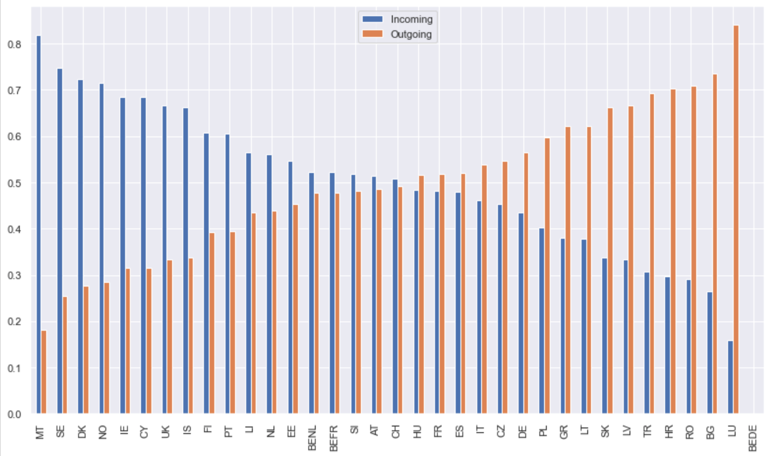
Ratio of incoming and outgoing students for each country
The country where I was born, Spain, it’s one of the most desired destinations for European students going abroad. Nevertheless, a lot of Spanish students go on an Erasmus too, like I did, so the proportion is quite balanced. However, there are countries that send a lot of students abroad, but barely receive any, and vice versa. With a bar plot, we can easily see the sending/receiving ratio for each country.
Analyzing Correlations Between Variables
Home and host country
The home and destination countries are categorical variables, not numeric, so calculating a correlation index wouldn’t be straightforward. For this reason, we opted for something more visual, like a heatmap.

In the heatmap above, each row represents a home country and each column a destination. The results are normalized for each home country, meaning that the colors represent the percentage of students from each country (rows) that chose each of the destinations (columns). From that chart, it looks like the entropy of this pair of variables is quite low, meaning that for a specific home country, it’s quite predictable which will be the preferred destinations. Let’s check it for one country:

If there were no correlation between the home and destination countries, for each home country, each destination country would receive 2.86% of the students. However, both in the heatmap and the pie chart above, it does not look like so. For instance, in the pie chart we can see how Spanish students have a huge preference for Italy (21.3%), France (12.4%), Germany (11.1%), UK (9.4%), Portugal (6.8%) and Poland (6.6%).
Destination and subject area
There are very prestigious universities around Europe, but it’s very difficult to find one that excels in every knowledge area. For that reason, it would be interesting to find out if for each subject area, there is a preference towards some institutions over others. Since we’re dealing again with categorical variables, let’s apply the same technique as before.
If the correlation between the subject area and the destination university were null, for each subject area, each destination university would receive 0.04% of the students. However, for most of the subject areas, the institution receiving more students has between a 1% and 3.7%, showing that the entropy between those two variables is not high. However, in this sense, we couldn’t find any university highlighting over the rest. The percentages for the “General” category are remarkable, with only three institutions receiving almost the 50% of the students.
Home and host country and monthly grant
When I was doing the paperwork for my Erasmus exchange in 2019, I remember that the Spanish government set three groups of destination countries according the cost of life, giving a different monthly grant for each of them. Once I was there, I was surprised to see how some friends coming from other European countries received more or less money than I did. Then, what does the monthly grant depend on: the country you’re going to, or the one you’re coming from? Let’s find it out!

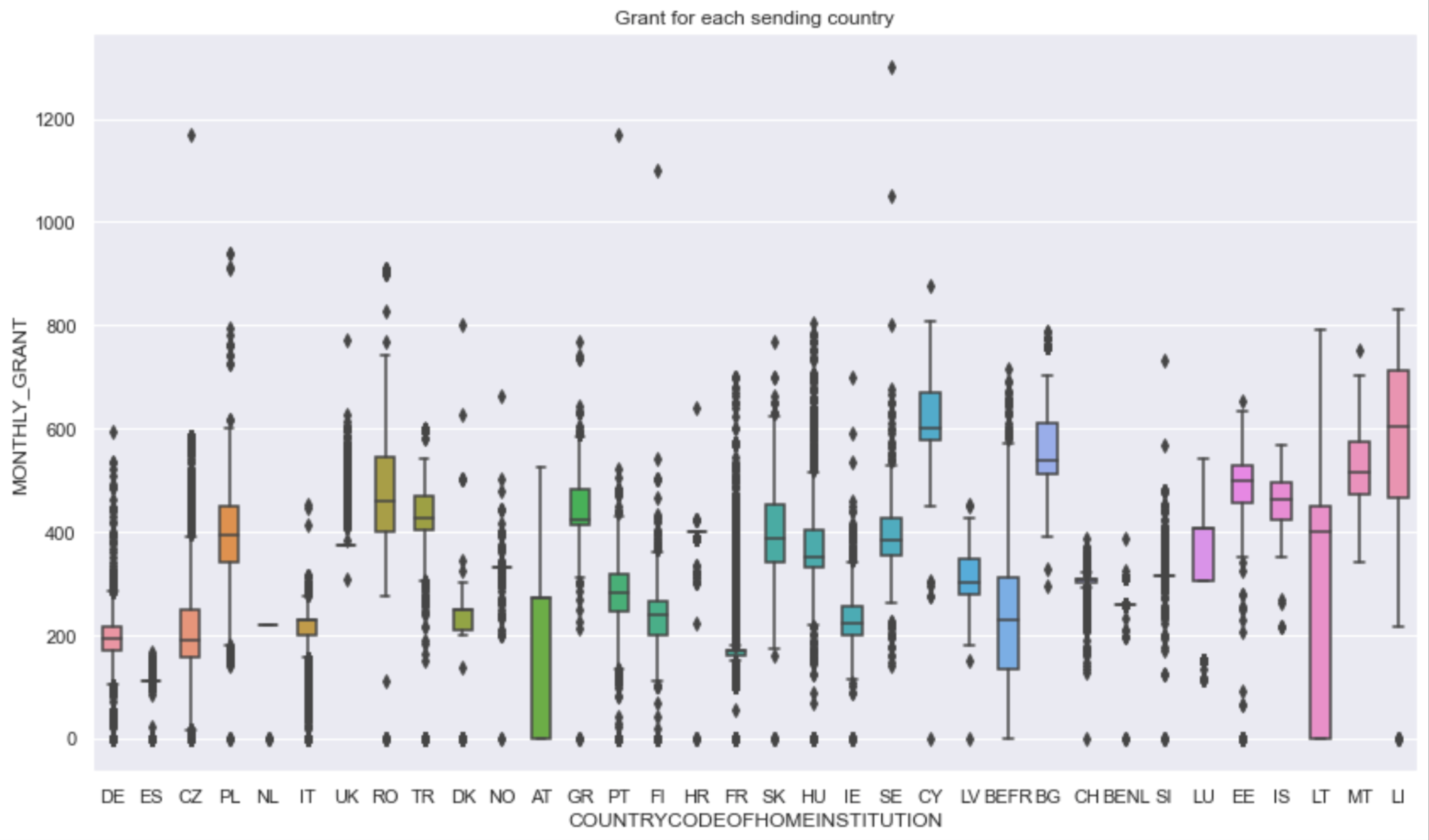
Comparing the two plots and obviating the enormous amount of outliers, it’s evident that the home country is a more deterministic factor than the destination country in the amount of money received by the students. In the first plot, it looks like the average of the monthly grant for each destination country is quite homogenous, and for most of them, the variance is very high, ranging from a 50% to a 150% of the average value, while in the second plot, the variance is really low, and the average grants are very heterogenous. Therefore, as I supposed before doing this analysis, the monthly grant depends mostly in the country you come from.
I hope that the post wasn’t too long for you. In fact, in this post I skipped some insights we made, to not make it too long, so if you’re interested, here you have the complete notebook. I would also like to give a shout-out again to Hilke van Meurs for the work put into this project. And of course, if you have any question or suggestion, please let me know in the comments.
Reference
- JupyterLab: https://jupyter.org/install
- Pandas DataFrame: https://pandas.pydata.org/pandas-docs/stable/reference/api/pandas.DataFrame.html
- Matplotlib: https://matplotlib.org/api/
- Erasmus 2011–12 Datasets: https://data.europa.eu/euodp/en/data/dataset/erasmus-mobility-statistics-2011-12
- Jupyter Notebook in GitHub: https://github.com/gbarreiro/erasmus-data-analysis/blob/main/Erasmus.ipynb