I always liked city maps and a few weeks ago I decided to build my own artistic versions of it. After googling a little bit I discovered this incredible tutorial written by Frank Ceballos. It is a fascinating and handy tutorial, but I prefer a more detailed/realistic blueprint maps. Because of that, I decided to build my own version. So let’s see how we can create beautiful maps with a little python code and OpenStreetMap data.
Installing OSMnx
First of all, we need tohave a Python installation. I recommend using Conda and virtual environments (venv) for achieving a tidy workspace. Moreover, we are going to use OSMnx Python package that will let us download spatial data from OpenStreetMap. We can accomplish the creation of a venv and installing OSMnx just writing two Conda commands:
After successfully install OSMnx, we can start coding. The first thing we need to do is to download the data. Downloading the data can be achieved in different ways, one of the easiest ways is to use graph_from_place().
Downloading Berlin street network
graph_from_place()has several parameters. placeis the query that is going to be used in OpenStreetMaps to retrieving the data, retain_allwill give us all the streets even if they are not connected to other elements, simplifyclean a little bit the returned graph and network_typespecify what type of street network to get.
I am looking to retrieve allpossible data but you can also download only drive roads, using drive, or pedestrian pathways using walk.
Another possibility is to use graph_from_point()that allows us to specify a GPS coordinate. This option is more in handy in multiple cases, like places with common names, and gives us more precision. Using distwe can retain only those nodes within this many meters of the centre of the graph.
Downloading Madrid street network
Also, it is necessary to take into account that if you are downloading data from bigger places like Madrid or Berlin, you will need to wait a little bit in order to retrieve all the information.
Unpacking and colouring our data
Both graph_from_place() and graph_from_point() will return a MultiDiGraph that we can unpack and store in the list as shown in Frank Ceballos tutorial.
Reaching this point we just need to iterate over data and colour it. We can colour it and adjust linewidths base on street lengths.
But there is also the possibility of identifying certain roads and only colour them differently.
In my example, I am only using colourMap.py Gist with the following colours.
color = “#a6a6a6”
color = “#676767”
color = “#454545”
color = “#bdbdbd”
color = “#d5d5d5”
color = “#ffff”
But feel free of changing the colours or conditions in order to create new maps that suit your taste.
Plot and save the map
Finally, we only need one thing left that is plotting the map. First, we need to identify the centre of our map. Choose the GPS coordinates where you want to be the centre. Then we will add some borders and background colour, bgcolor. north, south, eastand westwest will be new borders of our map. This coordinates will crop the image base on these boundaries, just increase the boundaries in you want a bigger map. Take into account that if you are using graph_from_point() method you will need to increase the dist value base on your needs. For bgcolor I am choosing a blue a dark blue #061529, to simulate a blueprint, but again you can adjust this to your liking.
After that, we just need to plot and save the map. I recommend use fig.tight_layout(pad=0) to adjust the plot params so that subplots are nicely fit.
Results
Using this code we can build the following examples but I recommend that you tunning your settings like line widths or border limit for each city.
Madrid City Map — Poster size
One difference to take into account between graph_from_place() and graph_from_point() it is that graph_from_point() will obtain street data from the surroundings, base on the dist that you set. Depending on if you want a simple map or a more detailed one you can exchange between them. The Madrid city map has been created using graph_from_place() and the Berlin city map has been created using graph_from_point() .
Berlin City Map
On top of that perhaps you want a poster size image. One easy way to accomplish that is to set figsizeattribute inside ox.plot_graph() .figsize can adjust the width, height in inches. I usually chose a bigger size like figsize=(27,40) .
Bonus: Add Water
OpenStreetMap has also data from rivers and other natural water sources, like lakes or water canals. Again using OSmnx we can download this data.
Downloading natural water sources
In the same way as before we can iterate over this data and colour it. In this case, I prefer blue colours like #72b1b1 or #5dc1b9.
Finally, we just need to save the figure. In this case, I am not using any borders with bbox inside plot_graph . That’s another thing that you can play with.
After successfully downloading rivers and like we just need to join the two images. Just a little Gimp or Photoshop will do the trick, remember to create the two images with the same fig_size or limit borders, bbox , for easier interpolation.
Berlin natural water sources
Finishing touches
One thing that I like to add is a text with the name of the city, GPS coordinates and the country name. Once more Gimp or Photoshop will do the trick.
Also if you add water you will need to fill some spaces or paint other water sources, like seawater. The line with of the rivers is not constant but using the paint bucket tool you can fill those gaps.
Code and conclusions
The code for creating these maps is available on my GitHub. Feel free to use it and show me your results!! Hope you liked this post and again thanks to Frank Ceballos and the Medium community. Additionally, if any of you want to print some posters I opened a little store on Etsy with my map creations.
Thanks for reading me and sharing knowledge will guide us to better and incredible results!!
Value-based Methods in Deep Reinforcement Learning
Deep Reinforcement learning has been a rising field in the last few years. A good approach to start with is the value-based method, where the state (or state-action) values are learned. In this post, a comprehensive review is provided where we focus on Q-learning and its extensions.
A Short Introduction to Reinforcement Learning (RL)
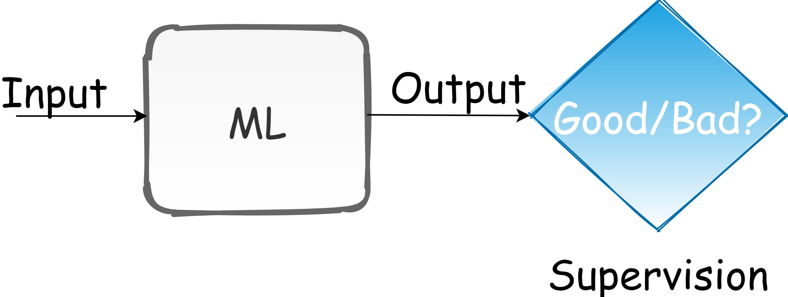
There are three types of common machine learning approaches: 1) supervised learning, where a learning system learns a latent map based on labeled examples, 2) unsupervised learning, where a learning system establishes a model for data distribution based on unlabeled examples, and 3) Reinforcement Learning, where a decision-making system is trained to make optimal decisions. From the designer’s point-of-view, all kinds of learning are supervised by a loss function. The sources of supervision must be defined by humans. One way to do this is by the loss function.
Image by author
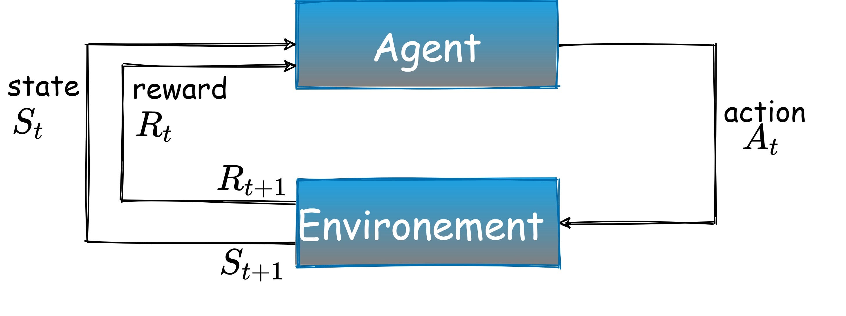
In supervised learning, the ground truth label is provided. But, in RL, we teach an agent by exploring the environment. We should design the world where the agent is trying to solve a task. This design is related to RL. A formal RL framework definition is given by [1]
an agent acting in an environment. At every point in time, the agent observes the state of the environment and decides on an action that changes the state. For each such action, the agent is given a reward signal. The agent’s role is to maximize the total received reward.
RL Diagram (image by author)
So, how it works?
RL is a framework for learning to solve sequential decision-making problems by trial & error in a world that provides occasional rewards. This is the task of deciding, from experience, the sequence of actions to perform in an uncertain environment to achieve some goals. Inspired by behavioral psychology, reinforcement learning (RL) proposes a formal framework for this problem. An artificial agent may learn by interacting with its environment. Using the experience gathered, the artificial agent can optimize some objectives given via cumulative rewards. This approach applies in principle to any type of sequential decision-making problem relying on past experience. The environment may be stochastic, the agent may only observe partial information about the current state, etc.
Why go deep?
Over the past few years, RL has become increasingly popular due to its success in addressing challenging sequential decision-making problems. Several of these achievements are due to the combination of RL with deep learning techniques. For instance, a deep RL agent can successfully learn from visual perceptual inputs made up of thousands of pixels (Mnih et al., 2015 / 2013).
“One of the most exciting fields in AI. It’s merging the power and the capabilities of deep neural networks to represent and comprehend the world with the ability to act and then understanding the world”.
It has solved a wide range of complex decision-making tasks that were previously out of reach for a machine. Deep RL opens up many new applications in healthcare, robotics, smart grids, finance, and more.
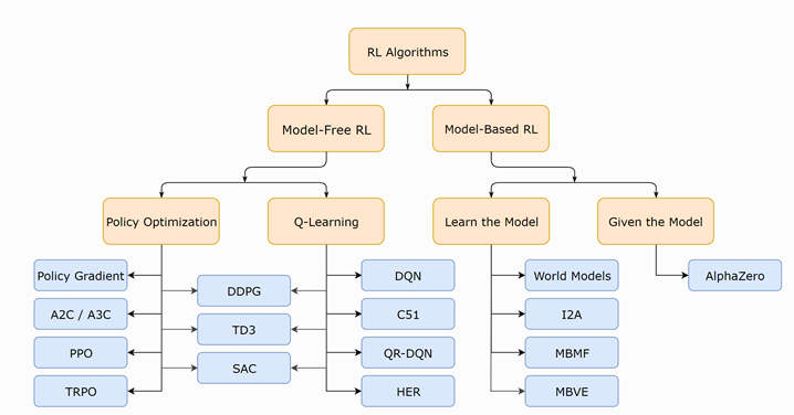
Types of RL
Value-Based: learn the state or state-action value. Act by choosing the best action in the state. Exploration is necessary. Policy-Based: learn directly the stochastic policy function that maps state to action. Act by sampling policy. Model-Based: learn the model of the world, then plan using the model. Update and re-plan the model often.
Mathematical background
We now focus on the value-based method, which belongs to “model-free” approaches, and more specifically, we will discuss the DQN method, which belongs to Q-learning. For that, we quickly review some necessary mathematical background.
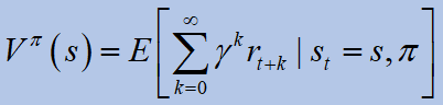
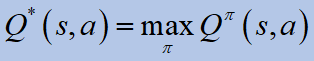
An RL agent goal is to find a policy such that it optimizes the expected return (V-value function):
where Eis the expected value operator, gamma is the discount factor, and pi isa policy. The optimal expected return is defined as:
The optimal V-value function is the expected discounted reward when in a given statesthe agent follows the policypi* thereafter.
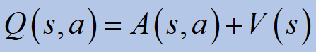
2. Q value
There are more functions of interest. One of them is the Quality Value function:
Similarly to the V-function, the optimal Q value is given by:
The optimal Q-value is the expected discounted return when in a given state s and for a given action, a,the agent follows the policy pi* thereafter. The optimal policy can be obtained directly from this optimal value:
3. Advantage function
We can relate between the last two functions:
It describes “how good” the action ais, compared to the expected return when following direct policy pi.
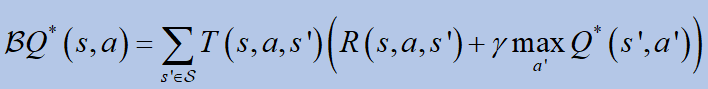
4. Bellman equation
To learn the Q value, the Bellman equation is used. It promises a unique solution Q*:
where B is the Bellman operator:
To promise optimal value: state-action pairs are represented discretely, and all actions are repeatedly sampled in all states.
Q-Learning
Q learning in an off-policy method learns the value of taking action in a state and learning Q value and choosing how to act in the world. We define state-action value function: an expected return when starting in s, performing a, and following pi. Represented in a tabulated form. According to Q learning, the agent uses any policy to estimate Q that maximizes the future reward. Q directly approximates Q*, when the agent keeps updating each state-action pair.
For non-deep learning approaches, this Q function is just a table:
Image by author
In this table, each of the elements is a reward value, which is updated during the training such that in steady-state, it should reach the expected value of the reward with the discount factor, which is equivalent to the Q* value. In real-world scenarios, value iteration is impractical;
Image by Google
In the Breakout game, the state is screen pixels: Image size: 84×84, Consecutive: 4 images, Gray levels: 256. Hence, the number of rows in the Q-table is:
Just to mention, in the universe, there are 10⁸² atoms. This is a good reason why we should solve problems like the Breakout game in deep reinforcement learning…
DQN: Deep Q-Networks
We use a neural network to approximate the Q function:
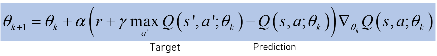
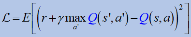
The neural network is good as a function approximator. DQN was used in the Atari games. The loss function has two Qs functions:
Target: the predicted Q value of taking action in a particular state. Prediction: the value you get when actually taking that action (calculating the value on the next step and choosing the one that minimizes the total loss).
Parameter updating:
When updating the weights, one also changes the target. Due to the generalization/ extrapolation of neural networks, large errors are built in the state-action space. Hence, the Bellman equation is not converged w.p. 1. Errors may propagate with this update rule (slow / unstable/ etc.).
DQN algorithm can obtain strong performance in an online setting for a variety of ATARI games and directly learns from pixels. Two heuristics to limit the instabilities: 1. The parameters of the target Q-network are updated only every N iterations. This prevents the instabilities from propagating quickly and minimizes the risk of divergence.2. The experience replay memory trick can be used.
DQN Architecture (MDPI: Comprehensive Review of Deep Reinforcement Learning Methods and Applications in Economics)
DQN Tricks: experience replay and epsilon greedy
Experience replay
in DQN, a CNN architecture is used. The approximation of Q-values using non-linear functions is not stable. According to the experience replay trick: all experiences are stored in a replay memory. When training the network, random samples from the replay memory are used instead of the most recent action. In different words: the agent collects memories\stores experience (state transitions, actions, and rewards) and creates mini-batches for the training.
Epsilon Greedy Exploration
As the Q function converges to Q*, it actually settles with the first effective strategy it finds. Hence, exploration is greedy. An effective way to explore is by choosing a random action with probability “epsilon” and other-wise (1-epsilon), go with the greedy action (with highest Q value). The experience is collected by the epsilon-greedy policy.
DDQN: Double Deep Q-Networks
The max operator in Q-learning uses the same values both to select and evaluate action. It makes it more likely to select overestimated values (in case of noise or inaccuracies), resulting in overoptimistic value estimates. In DDQN, there is a separate network for each Q. Hence, there are two neural networks. It helps reduces bias where policy is still chosen according to the values obtained by the current weights.
Tow neural networks, with Q function for each:
Now, the loss function is provided by:
Dueling Deep Q-Networks
Q contains advantage (A)value in addition to the value (V) of being in that state. A is defined earlier as the advantage of taking action a in state s among all other possible actions and states. If all the actions you aim to take are “pretty good”, we want to know: how better it is?
The dueling network represents two separate estimators: one for the state value function and one for the state-dependent action advantage function. For further reading with code example, we refer to the dueling-deep-q-networks post by Chris Yoon.
Summary
We presented the Q-learning in value-based method, with a general introduction for reinforcement learning and motivation to put it in the deep learning context. A mathematical background, DQN, DDQN, some tricks, and the dueling DQN have been explored.
About the author
Barak Or received the B.Sc. (2016), M.Sc. (2018) degrees in aerospace engineering, and also B.A. in economics and management (2016, Cum Laude) from the Technion, Israel Institute of Technology. He was with Qualcomm (2019–2020), where he mainly dealt with Machine Learning and Signal Processing algorithms. Barak currently studies toward his Ph.D. at the University of Haifa. His research interest includes sensor fusion, navigation, machine learning, and estimation theory.
[1] Sutton, Richard S., and Andrew G. Barto. Reinforcement learning: An introduction. MIT Press, 2018.
[2] Human-level control through deep reinforcement Learning, Volodymyr Mnih et al., 2015. on Nature.
[3] Mosavi, Amirhosein, et al. “Comprehensive review of deep reinforcement learning methods and applications in economics.” Mathematics 8.10 (2020): 1640.
[4] Baird, Leemon. “Residual algorithms: Reinforcement learning with function approximation.” Machine Learning Proceedings 1995. Morgan Kaufmann, 1995. 30–37.
This post is a followup to my deep dive on the mechanics of uplift modeling, with a worked example. Here I describe how we on the Data Science team at Tala applied uplift modeling to help past-due borrowers repay their loans. Tala offers the world’s most accessible consumer credit product, instantly underwriting and then disbursing loans to people who have never had a formal credit history, all through a smartphone app.
Introduction
Of the many ways that machinelearning can create value for businesses, uplift modeling is one of the lesser known. But for many use cases, it may be the most effective modeling technique. In any situation where there is a costly action a business can selectively take for different customers, in hopes of influencing their behavior, uplift modeling should be a strong candidate for finding that subset of customers that would be most influenced by the action. This is important for maximizing the return on investment in a business strategy.
In this post, I’ll outline the business problem we tackled with uplift modeling at Tala, the basics of uplift models and how we built one, how the predictions of uplift models can be explained, how the uplift concept can be extended to provide direct financial insights, and considerations for monitoring the performance of uplift models in production.
Use case at Tala: past-due borrowers
When borrowers go past due on their loans, they put their own financial health at risk, as well as the health of the business that lent to them. One of Tala’s primary means for reaching out to past-due borrowers and encouraging them to repay their loans is via telephone. However, this is an expensive process and must be balanced with the expected increase in revenue that a phone call will bring: how much more likely is it that a borrower will make a payment if we call them?
Mathematically, we are interested in the uplift in probability of payment due to calling a borrower. This is defined as the difference in probability of payment if the borrower is called, versus if they aren’t called.
Image by author
The premise of uplift modeling is that it can help us identify the borrowers who will have the biggest increase in repayment probability if given a phone call. In other words, those who are more persuadable. If we can identify these borrowers, we can more effectively prioritize our resources to maximize both borrowers’ and Tala’s financial health.
Focusing on the opportunity
Now that we know the goal of uplift modeling, how do we get there? Uplift modeling relies on randomized, controlled experiments: we need a representative sample of all different kinds of borrowers in both a treatment group, who received a phone call, as well as a control group that wasn’t called.
Once we obtained this data set, we observed that the fraction of borrowers making a payment was significantly higher in the treatment group than the control group. This provided evidence that phone calls were “working” in the sense that they effectively encouraged repayment on average across all borrowers. This is called the average treatment effect (ATE). Quantifying the ATE is the typical outcome of an A/B test.
However, it may be that only a portion of borrowers within the treatment group were responsible for most of the ATE we observed. As an extreme example, maybe half of the borrowers in the treatment group were responsible for the entire ATE. If we had some way to identify this segment of borrowers ahead of time, who would more readily respond to treatment, then we would be able to concentrate our telephonic resources on them, and not waste time on those for whom phone calls have little or no effect. We may need to find other ways to engage the non-responders. The process of determining variable treatment effects from person to person, conditional on the different traits these people have, means we’re looking for the conditional average treatment effect (CATE). This is where machine learning and predictive modeling come into the picture.
Building and explaining the uplift model
In machine learning, we can describe the differences between borrowers via features, which are various quantities specific to a borrower. We engineered features related to borrowers’ history of payment, as well as results of past phone calls and interactions with the Tala app. The features attempt to characterize a borrower’s willingness and capacity to repay, as well as their commitment to establishing and maintaining a relationship with Tala. Will the borrower listen to and learn from us, and give us the opportunity to do the same with them?
Armed with the features and modeling framework described above, we were ready to build our uplift model. We used an approach called the S-Learner. For details on this, see my previous blog post on uplift modeling. Once the S-Learner was built and tested, we trained a separate regression model on the training set with a target variable of uplift (the difference in predicted probabilities given treatment and no treatment), and the same features used to train the S-Learner (except for the treatment flag, which is considered a feature in the S-Learner approach). Using the testing set SHAP values from this regression model, we were able to gain insight into which model features had the largest impact on predictions of uplift.
Although the feature names are anonymized here, the interpretation of the most predictive features all made sense in that the borrowers who demonstrate willingness to pay, have experience with borrowing and may want to borrow again, and are receptive to telephonic outreach, are the kinds of borrowers worth encouraging to repay via phone calls.
SHAP values for the uplift model, indicating the top five anonymized factors influencing predictions. Features were based on payment and phone call history of borrowers. Image by author.
Designing strategies to use and monitor the model
Knowing the predicted uplift in probability was the first step in our model-guided strategy. However, we are not just interested in how much more likely someone is to make a payment, but also the likely increase in the amount of payment due to phone outreach. To determine this, we combined the uplift in probability with information about the amount owed by a borrower and the likely amount of payment. This turned the predicted uplift in probability into an estimate of the revenue uplift due to the phone call, allowing us to rank borrowers on how valuable it would be to call them.
The opportunity represented by ranking borrowers on predicted revenue uplift can be seen by calculating the actual revenue uplift, as the difference in average revenue between treatment and control groups, for different bins of predicted revenue uplift. Such an analysis is analogous to the idea of an uplift decile chart detailed here. We used the model testing set for this.
Revenue uplift decile chart: Difference in average revenue between treatment and control when ranking accounts by predicted revenue uplift. Image by author.
The results show that predicted revenue uplift effectively identifies accounts where phone calls are of more value. Over half of the incremental revenue available by calling all borrowers can be obtained by calling only the top 10% of borrowers ranked in this way, and 90% of the incremental revenue can be had by calling the top half of borrowers. In fact, when considering the average cost of telephonic outreach per borrower, shown as a green line, it’s apparent that only the top 50% of borrowers are profitable to call.
Given the apparent opportunity in using predicted revenue uplift to guide telephonic outreach, we deployed this model to guide our strategy. To monitor model performance after deployment, we created two groups that would enable us to examine the true uplift of phone calls, across the full range of predicted uplift. We did this by calling a randomly selected 5% of borrowers, no matter what their predicted uplift was, and not calling another 5%. Based on the results from these tests, we were able to conclude that the model was functioning as intended in production, using the same kind of model assessment metrics shown here and in my companion blog post.
In conclusion, uplift modeling allowed Tala to focus repayment efforts on borrowers who would be most receptive to those efforts, saving time and money. I hope you find this account of Tala’s experience with uplift modeling helpful for your work.
Originally published at https://tala.co on January 14, 2021.
As deep learning methodologies have developed, it has been generally agreed that increasing the size of a neural network improves performance. However, this is at the detriment of memory and compute requirements, which also need to be increased to train the model.
This can be put into perspective by comparing the performance of Google’s pre-trained language model, BERT, at different architecture sizes. In the original paper, Google’s researchers reported an average GLUE score of 79.6 for BERT-Base and 82.1 for BERT-Large. This small increase of 2.5 came with an extra 230M parameters (110M vs. 340M)!
As a rough calculation, if each parameter is stored in single precision (more detail below), which is 32 bytes of information, then 230M parameters is equivalent to 0.92Gb in memory. This may not seem too large in and of itself, but consider that during each training iteration these parameters goes through a series of steps of matrix arithmetics, calculating further values, such as gradients. All these extra values can quickly become unmanageable.
In 2017, a group of researchers from NVIDIA released a paper detailing how to reduce the memory requirements of training neural networks, using a technique called Mixed Precision Training:
We introduce methodology for training deep neural networks using half-precision floating point numbers, without losing model accuracy or having to modify hyperparameters. This nearly halves memory requirements and, on recent GPUs, speeds up arithmetic.
In this article, we will explore mixed-precision training, understanding both how it fits into the standard algorithmic framework of deep learning and how it is able to reduce computational demand without affecting model performance.
Floating Point Precision
The technical standard used for representing floating-point numbers in binary formats is IEEE 754, established in 1985 by the Institute of Electrical and Electronics Engineering.
As set out in IEEE 754, there are various levels of floating-point precision, ranging from binary16 (half-precision) to binary256 (octuple-precision), where the number after “binary” equals the number of bits available for representing the floating-point value.
Unlike integer values, where the bits simply represent the binary form of the number, perhaps with a single bit reserved for the sign, floating-point values also need to consider an exponent. Therefore, the representation of these numbers in binary form is more nuanced and can significantly affect precision.
Historically, deep learning has used single-precision (binary32, or FP32) to represent parameters. In this format, one bit is reserved for the sign, 8 bits for the exponent (-126 to +127) and 23 bits for the digits. Half-precision, or FP16, on the other hand, reserves one bit for the sign, 5 bits for the exponent (-14 to +14) and 10 for the digits.
Comparison of the format for FP16 (top) and FP32 (bottom) floating-point numbers. The number shown, for illustrative purposes, is the largest number less than one that can be represented by each format. Illustration by author.
However, this comes at a cost. The smallest and largest positive, normal values for each are as follows:
As well as this, smaller denormalized numbers can be represented, where all the exponent bits are set to zero. For FP16, the absolute limit is 2^(-24) However, as denormalized numbers get smaller, the precision decreases.
We will not go into any further depth here to understand the quantitative limitations of different floating-point precision in this article, but the IEEE provides comprehensive documentation for further investigation.
Mixed Precision Training
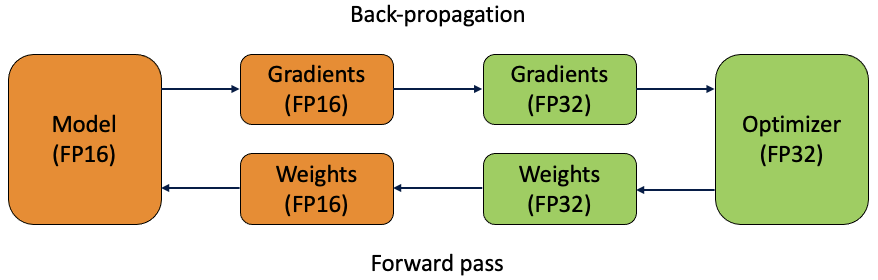
During standard training of neural networks FP32 to represent model parameters at the cost of increased memory requirements. In mixed-precision training, FP16 is used instead to store the weights, activations and gradients during training iterations.
However, as we saw above this creates a problem, as the range of values that can be stored by FP16 is smaller than FP32, and precision decreases as number become very small. The result of this would be a decrease in the accuracy of the model, in line with the precision of the floating-point values calculated.
To combat this, a master copy of the weights is stored in FP32. This is converted into FP16 during part of each training iteration (one forward pass, back-propagation and weight update). At the end of the iteration, the weight gradients are used to update the master weights during the optimizer step.
Mixed precision training converts the weights to FP16 and calculates the gradients, before converting them back to FP32 before multiplying by the learning rate and updating the weights in the optimizer. Illustration by author.
Here, we can see the benefit of keeping the FP32 copy of the weights. As the learning rate is often small, when multiplied by the weight gradients they can often be tiny values. For FP16, any number with magnitude smaller than 2^(-24) will be equated to zero as it cannot be represented (this is the denormalized limit for FP16). Therefore, by completing the updates in FP32, these update values can be preserved.
The use of both FP16 and FP32 is the reason this technique is called mixed-precision training.
Loss Scaling
Although mixed-precision training solved, in the most part, the issue of preserving accuracy, experiments showed that there were cases where small gradient values occurred, even before being multiplied by the learning rate.
The NVIDIA team showed that, although values below 2^-27 were mainly irrelevant to training, there were values in the range [2^-27, 2^-24) which were important to preserve, but outside of the limit of FP16, equating them to zero during the training iteration. This problem, where gradients are equated to zero due to precision limits, is known as underflow.
Therefore, they suggest loss scaling, a process by which the loss value is multiplied by a scale factor after the forward pass is completed and before back-propagation. The chain rule dictates that all the gradients are subsequently scaled by the same factor, which moved them within the range of FP16.
Once the gradients have been calculated, they can then be divided by the same scale factor, before being used to update the master weights in FP32, as described in the previous section.
During loss scaling, the loss is scaled by a predefined factor after the forward pass to ensure it falls within the range of representable FP16 values. Due to the chain rule, this scales the gradients by the same factor, so the actual gradients can be retrieved after back-propagation. Illustration by author.
In the NVIDIA “Deep Learning Performance” documentation, the choice of scaling factor is discussed. In theory, there is no downside to choosing a large scaling factor, unless it is large enough to lead to overflow.
Overflow occurs when the gradients, multiplied by the scaling factor, exceed the maximum limit for FP16. When this occurs, the gradient becomes infinite and is set to NaN. It is relatively common to see the following message appear in the early epochs of neural network training:
Gradient overflow. Skipping step, loss scaler 0 reducing loss scale to…
In this case, the step is skipped, as the weight update cannot be calculated using an infinite gradient, and the loss scale is reduced for future iterations.
Automatic Mixed Precision
In 2018, NVIDIA released an extension for PyTorch called Apex, which contained AMP (Automatic Mixed Precision) capability. This provided a streamlined solution for using mixed-precision training in PyTorch.
In only a few lines of code, training could be moved from FP32 to mixed precision on the GPU. This had two key benefits:
Reduced training time — training time was shown to be reduced by anywhere between 1.5x and 5.5x, with no significant reduction in model performance.
Reduced memory requirements — this freed up memory to increase other model elements, such as architecture size, batch size and input data size.
As of PyTorch 1.6, NVIDIA and Facebook (the creators of PyTorch) moved this functionality into the core PyTorch code, as torch.cuda.amp. This fixed several pain points surrounding the Apex package, such as version compatibility and difficulties in building the extension.
Although this article will not go any further into the code implementation of AMP, examples can be seen in the PyTorch documentation.
Conclusion
Although floating-point precision is often overlooked, it plays a key role in the training of deep learning models, where small gradients and learning rates multiply to create gradient updates that require more bits to be precisely represented.
However, as state-of-the-art deep learning models push the boundaries in terms of task performance, architectures grow and precision has to be balanced against training time, memory requirements and available compute.
Therefore, the ability of mixed precision training to maintain performance whilst essentially halving the memory usage is a significant advance in deep learning!
This week marks Holocaust Memorial Day and the end of my five years studying in the Statistics department of University College London (UCL), which was the home, for decades, of the most prominent eugenicists.
Until this week, it didn’t bother me that I studied the work of Karl Pearson and Ronald Fisher in the Galton Lecture Theatre and Pearson Building. But it should have done.
Much of my family was murdered in the holocaust as part of a regime to eradicate a supposed “inferior race”. Yet, I still viewed Pearson, Fisher, and Galton (and others) as the Fathers of Statistics who deserved to be recognised and respected for their contributions. I had naïvely assumed they were a product of their time and that their research was a natural progression in the statistics behind genetics. This was not the case.
Note: This is a personal article that I wrote in order to hold my own naïvety to account. However, this is aimed at other statisticians and data scientists as I am surely not the only person who failed to consider the true origins of our field.
Francis Galton, “the founder of the field of behavioral and educational statistics”:¹
Pioneered the use of questionnaires
Discovered regression to the mean
Re-discovered correlation and regression and discovered how to apply these in anthropology, psychology, and more
Defined the concept of standard deviation
Galton is considered so fundamentally important and critical to the development of statistics, that many will deliberately overlook his establishment of the field of Eugenics in 1883.
A product of his time?
In reviewing four books about the life of Galton, Clauser (2007)¹ uses this argument to criticise one book:
“The volume is also limited by Brookes’s tendency to see every aspect of Galton’s life in relation to his views on eugenics. Brookes fails to place Galton’s views in the context of the times in which he lived…Although Galton’s views of the indigenous populations that he encountered in Africa might well be seen as enlightened by Victorian standards, Brookes views them with a 21st-century perspective and finds evidence of Galton’s intolerance.”
The ‘product of its time’ argument is constantly used to justify bigotry throughout the years. To put this in perspective: Galton was inspired by his cousin’s work, The Origin of Species. Darwin could be called a product of his time as he used words like ‘savages’ to describe certain populations. However, Darwin spoke openly against racism and did not promote or contribute to any of Galton’s work on eugenics.² If there is any doubt about the innate racism in Galton’s ‘eugenics’, below is his reasoning for coining the term:
We greatly want a brief word to express the science of improving stock, which…takes cognisance of all influences that tend in however remote a degree to give the more suitable races or strains of blood a better chance of prevailing speedily over the less suitable than they otherwise would have had.³
And if there is still some doubt about Galton’s views, he also wrote:
There exists a sentiment, for the most part quite unreasonable, against the gradual extinction of an inferior race.⁴
If, on my first day of university, sitting in the Galton Lecture Theatre, I had been told that Galton felt that genocide was ‘for the most part quite unreasonable’, I may have felt less comfortable with his name and picture around me. My research fundamentally relies on Galton’s work, I am indebted to Galton. That does not mean I needed to hear and say his name every day for three years.
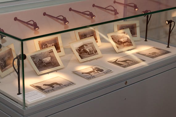
The Galton Exhibition held at UCL to raise awareness of their contribution to Eugenics. Credit: UCL Image Store.⁵
Karl Pearson
Karl Pearson was Galton’s protégé and amongst many notable achievements:
Developed hypothesis testing
Developed the use of p-values
Defined the Chi-Squared test
Introduced the Method of Moments
An antisemite
In the year Mein Kampf was published, Pearson wrote about the Jewish population:
“[they] will develop into a parasitic race…Taken on the average, and regarding both sexes, this alien Jewish population is somewhat inferior physically and mentally to the native population.”⁶
And when Hitler was made Chancellor, Pearson made a point to say:
Even at the present day there are far too many general impressions drawn from limited or too often wrongly interpreted experience, and far too many inadequately demonstrated and too lightly accepted theories for any nation to proceed hastily with unlimited Eugenic legislation.⁷
Which may appear reasonable until immediately followed by his caveat:
This statement, however, must never be taken as an excuse for indefinitely suspending all Eugenic teaching and every form of communal action in matters of sex.⁷
I concluded my undergraduate with a presentation, that fundamentally depended on the work of Pearson, in a small classroom in the Pearson building. Pearson, the first Chair of the Department of Eugenics at UCL, has contributed to my life and my work in a way that I cannot and will not ignore. His contributions were essential to the field of Statistics, and many others. But again I am left wondering if I would have felt as comfortable walking through the Pearson building, if I had been provided more context about the man it was named after.
UCL’s Pearson Building (left), 1985.⁸ Credit: UCL Image Store.
Sir Ronald Fisher
Fisher’s work in statistics established and promoted many important methods of statistical inference. His contributions include:
Establishing p = 0.05 as the normal threshold for significant p-values
Promoting Maximum Likelihood Estimation
Developing the ANalysis Of VAriance (ANOVA)
The iris dataset (this seems an incredibly minor contribution but I use it daily)⁹
Like Pearson and Galton, Fisher was revered. When asked who the “greatest biologist since Darwin” was, Richard Dawkins nominated Fisher¹⁰ (this may not be surprising given Dawkins’ own publicised views). Bodmer, one of Fisher’s students wrote a brief but glowing biography of Fisher’s life and described Fisher as “sweet” and “nice”.¹¹ Neither mentioned eugenics.
On the Nazi eugenicist Otmar Freiherr von Verschuer, Fisher wrote:
In spite of their prejudices I have no doubt also that the Party sincerely wished to benefit the German racial stock, especially by the elimination of manifest defectives, such as those deficient mentally, and I do not doubt that von Verschuer gave, as I should have done, his support to such a movement.¹²
I did not come across Fisher’s name until my third year at UCL, once again lauded as a great statistician. Needless to say, genocide was not discussed.
Buildings and Statements
As put in a recent article, discussing buildings named after people:
The right way to understand them and their ideas is through a properly contextualised display in a museum, not through an uncommented memorial that conceals more than it reveals.¹³
The same is true of sweeping statements about people. I assume that when Dawkins described Fisher as the “greatest biologist since Darwin”, this was based on pure output and contributions to the field alone. However the word “greatest”, like a building named after Fisher, includes judgement about the person itself. It implicitly assumes this person was “great” and we automatically assume (though this is not part of the definition) that “great” means “good”. Sweeping statements, as with uncommented memorials, conceal more than they reveal.
The Fathers of Statistics and Eugenics
Denaming buildings and lecture theatres is easy. It’s a step that should have been taken a long time ago, but I am not criticising UCL. To their credit, they spent years gathering information and putting out surveys to hear everyone’s feedback and opinions.
To work in statistics or data science is to work in the shadow of eugenics. For five years, I was not even aware that I was under this shadow and I am deeply ashamed. But I cannot blame myself. I used the equations I was provided and studied the methods I was told, I didn’t consider the names belonging to the methods. I believe I am likely in the majority with other mathematicians and statisticians. This is not okay. I believe that all Statistics courses should include, at the very least, one lecture on the full history of Statistics and its “Fathers”.
Success from failure
Even when buildings are renamed, I will still (daily) be using ‘Pearson’s Chi-Squared test’ and ‘Fisher’s information’. Their names are stuck with me forever and now so are their beliefs. Whilst I will respect and even be inspired by the contributions of these men to statistics, I can now talk about them without glorifying their characters or inadvertently condoning their beliefs. I will utilise the methods of the past to promote the positive, good, and ethical choices of the future. Learning where others failed will help generations of statisticians learn how to succeed.
Products of our time
Unfortunately, I can only end this on a warning. Whilst it is unlikely (though not impossible) that eugenics will re-emerge in modern politics, statistics and data are being manipulated now more than ever.
From naïve misuses of machine learning that return erroneous results, to the malicious manipulation of raw data, the field is being tested. From governments to individuals, Russia to Palo Alto, anti-maskers to anti-vaxxers; the full consequences of data and statistics malpractice remains unknown.
Sitting idly by as this happens will make us ‘a product of their time’. This is not good enough. Data Science needs more regulation. Doctors have the Hippocratic Oath, why don’t we have the Nightingale Oath: “Manipulate no data nor results. Promote ethical uses of statistics. Only train models you understand. Don’t promote Eugenics”.
Pandas is a highly popular data analysis and manipulation library for Python. It provides versatile and powerful functions to handle data in tabular form.
The two core data structures of Pandas are DataFrame and Series. DataFrame is a two-dimensional structure with labelled rows and columns. It is similar to a SQL table. Series is a one-dimensional labelled array. The labels of values in a Series are referred to as index. Both DataFrame and Series are able to store any data type.
In this article, wewill go through 20 examples that demonstrate various operations we can perform on a Series.
Let’s first import the libraries and then start with the examples.
import numpy as np
import pandas as pd
1. DataFrame is composed of Series
An individual row or column of a DataFrame is a Series.
Consider the DataFrame on the left. If we select a particular row or column, the returned data structure is a Series.
a = df.iloc[0, :]
print(type(a))
pandas.core.series.Seriesb = df[0]
type(b)
pandas.core.series.Series
2. Series consists of values and index
Series is a labelled array. We can access the values and labels which are referred to as index.
As we see in the previous example, an integer index starting from zero are assigned to a Series by default. However, we can change it using the index parameter.
ser = pd.Series(['a','b','c','d','e'], index=[10,20,30,40,50])print(ser.index)
Int64Index([10, 20, 30, 40, 50], dtype='int64')
4. Series from a list
We have already seen this in the previous examples. A list can be passed to the Series function to create a Series.
Another common way to create a Series is using a NumPy array. It is just like creating from a list. We only change the data passed to the Series function.
Since Series contains labelled items, we can access to a particular item using the label (i.e. the index).
ser = pd.Series(['a','b','c','d','e'])print(ser[0])
aprint(ser[2])
c
7. Slicing a Series
We can also use the index to slice a Series.
ser = pd.Series(['a','b','c','d','e'])print(ser[:3])
0    a
1    b
2    c
dtype: object
print(ser[2:])
2    c
3    d
4    e
dtype: object
8. Data types
Pandas assigns an appropriate data type when creating a Series. We can change it using the dtype parameter. Of course, an appropriate data type needs to be selected.
There are multiple ways to count the number of values in a Series. Since it is a collection, we can use the built-in len function of Python.
ser = pd.Series([1,2,3,4,5])len(ser)
5
We can also use the size and shape functions of Pandas.
ser.size
5ser.shape
(5,)
The shape function returns the size in each dimension. Since a Series is one-dimensional, we get the length from the shape function. Size returns the total size of a Series or DataFrame. If used on a DataFrame, size returns the product of the number of rows and columns.
10. Unique and Nunique
The unique and nunique functions return the unique values and the number of unique values, respectively.
ser = pd.Series(['a','a','a','b','b','c'])ser.unique()
array(['a', 'b', 'c'], dtype=object)ser.nunique()
3
11. Largest and smallest values
The nlargest and nsmallest functions return the largest and smallest values in a Series. We get the 5 largest or smallest values by default but it can be changed using the n parameter.
The value_counts function returns the number of occurrences of each unique value in a Series. It is useful to get an overview of the distribution of values.
ser = pd.Series(['a','a','a','b','b','c'])ser.value_counts()
a    3
b    2
c    1
dtype: int64
15. From series to list
Just like we can create a Series from a list, it is possible to convert a Series to a list.
We can count the number of missing values by chaining the sum function with the isna function.
ser.isna().sum()
2
18. Rounding up floating point numbers
In data analysis, we are most likely to have numerical values. Pandas is highly capable of manipulating numerical data. For instance, the round function allows for rounding the floating points numbers up to a specific decimal points.
We can apply logical operators to a Series such as equal, less than, or greater than. They return the Series with boolean values indicating the values that fit the specified condition with True.
We can apply aggregate functions on a Series such as mean, sum, median an so on. One way to apply them separately on a Series.
ser = pd.Series([1, 2, 3, 4, 10])ser.mean()
4
There is a better way if we need to apply multiple aggregate functions. We can pass them in a list to the agg function.
ser.agg(['mean','median','sum', 'count'])mean       4.0
median     3.0
sum       20.0
count      5.0
dtype: float64
Conclusion
We have done 20 examples that demonstrate the properties of Series and the functions to interact with it. It is just as important as DataFrame because a DataFrame is composed of Series.
The examples in this article cover a great deal of commonly used data operations with Series. There are, of course, more functions and methods to be used with Series. You can learn more advanced or detailed operations as you need them.
Thank you for reading. Please let me know if you have any feedback.
There’s a lot of hype behind the new Apple M1 chip. So far, it’s proven to be superior to anything Intel has offered. But what does this mean for deep learning? That’s what you’ll find out today.
The new M1 chip isn’t just a CPU. On the MacBook Pro, it consists of 8 core CPU, 8 core GPU, and 16 core neural engine, among other things. Both the processor and the GPU are far superior to the previous-generation Intel configurations.
I’ve already demonstrated how fast the M1 chip is for regular data science tasks, but what about deep learning?
Short answer — yes, there are some improvements in this department, but are Macs now better than, let’s say, Google Colab? Keep in mind, Colab is an entirely free option.
The article is structured as follows:
CPU and GPU benchmark
Performance test — MNIST
Performance test — Fashion MNIST
Performance test — CIFAR-10
Conclusion
Important notes
Not all data science libraries are compatible with the new M1 chip yet. Getting TensorFlow (version 2.4) to work properly is easier said than done.
You can refer to this link to download the .whl files for TensorFlow and it’s dependencies. This is only for macOS 11.0 and above, so keep that in mind.
The test you’ll see aren’t “scientific” in any way, shape or form. They only compare the average training time per epoch.
CPU and GPU benchmark
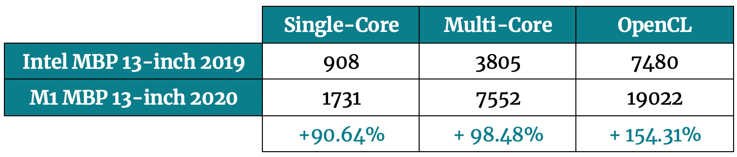
Let’s start with the basic CPU and GPU benchmarks first. The comparison is made between the new MacBook Pro with the M1 chip and the base model (Intel) from 2019. Geekbench 5 was used for the tests, and you can see the results below:
Image 1 — Geekbench 5 results (Intel MBP vs. M1 MBP) (image by author)
The results speak for themselves. M1 chip demolished Intel chip in my 2019 Mac. So far, things look promising.
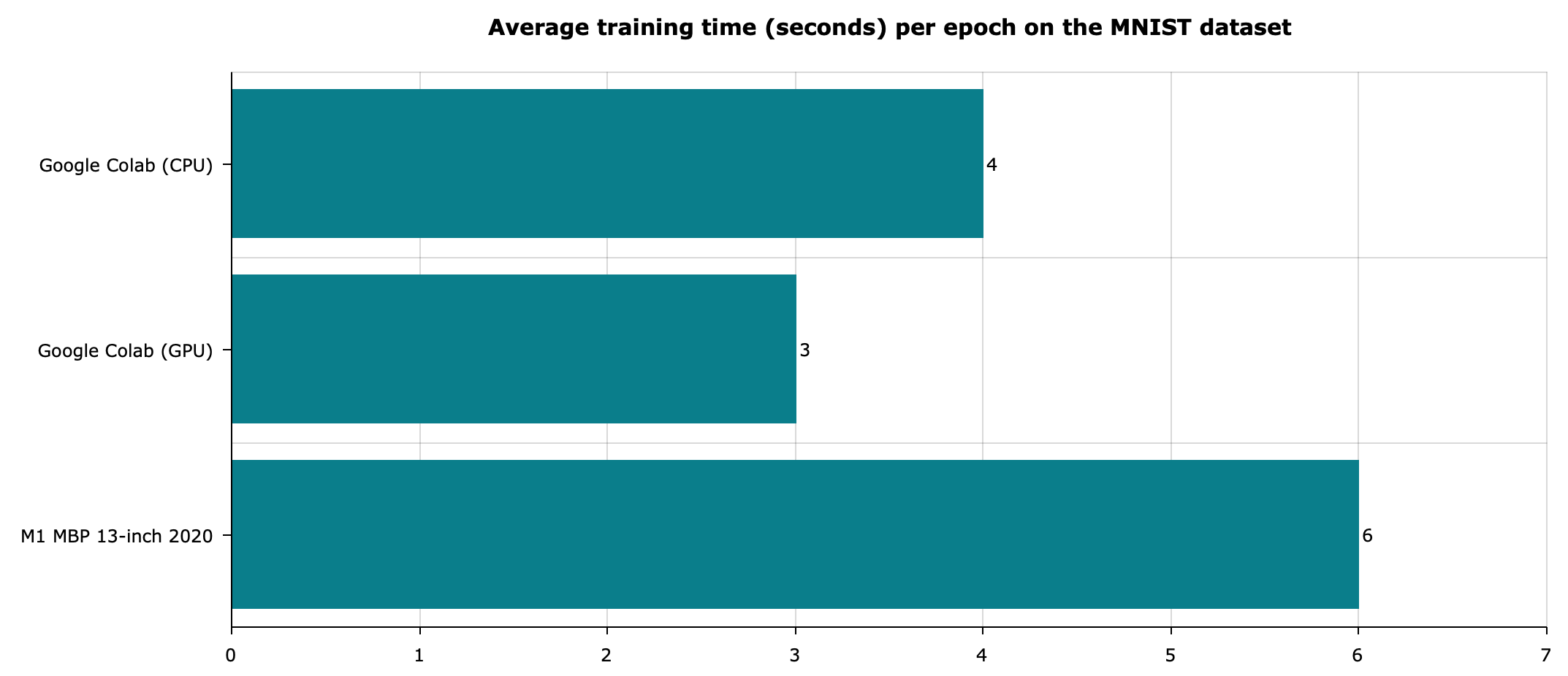
Performance test — MNIST
The MNIST dataset is something like a “hello world” of deep learning. It comes built-in with TensorFlow, making it that much easier to test.
The following script trains a neural network classifier for ten epochs on the MNIST dataset. If you’re on an M1 Mac, uncomment the mlcompute lines, as these will make things run a bit faster:
The above script was executed on an M1 MBP and Google Colab (both CPU and GPU). You can see the runtime comparisons below:
Image 2 — MNIST model average training times (image by author)
The results are somewhat disappointing for a new Mac. Colab outperformed it in both CPU and GPU runtimes. Keep in mind that results may vary, as there’s no guarantee of the runtime environment in Colab.
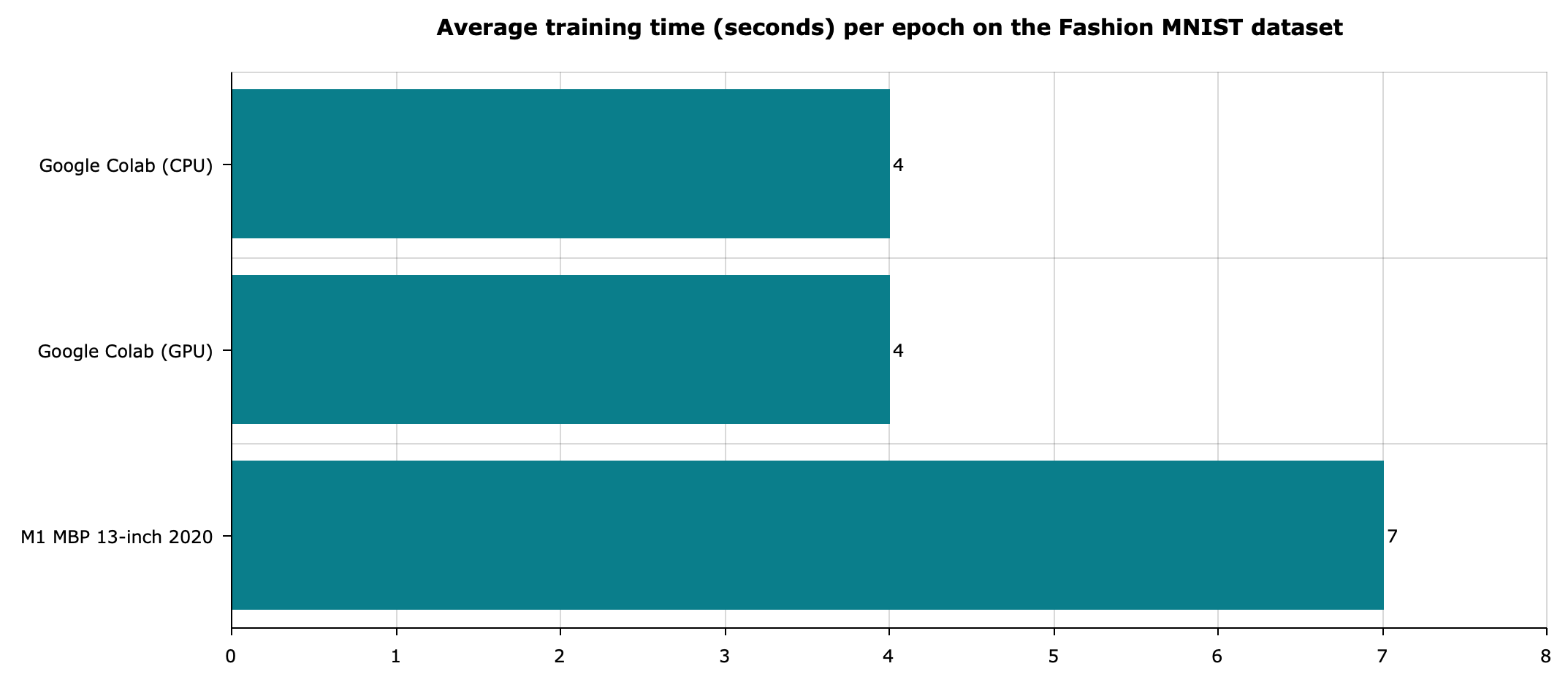
Performance test — Fashion MNIST
This dataset is quite similar to the regular MNIST, but is contains pieces of clothing instead of handwritten digits. Because of that, you can use the identical neural network architecture for the training:
As you can see, the only thing that’s changed here is the function used to load the dataset. The runtime results for the same environments are shown below:
Image 3 — Fashion MNIST model average training times (image by author)
Once again, we get similar results. It’s expected, as this dataset is quite similar to MNIST.
But what will happen if we introduce a more complex dataset and neural network architecture?
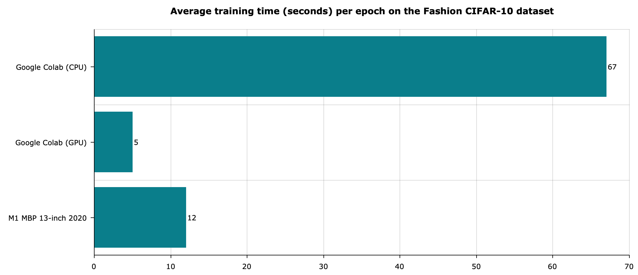
Performance test — CIFAR-10
CIFAR-10 also falls into the category of “hello world” deep learning datasets. It contains 60K images from ten different categories, such as airplanes, birds, cats, dogs, ships, trucks, etc.
The images are of size 32x32x3, which makes them difficult to classify even for humans in some cases. The script below trains a classifier model by using three convolutional layers:
Let’s see how convolutional layers and more complex architecture affects the runtime:
Image 4 — CIFAR-10 model average training times (image by author)
As you can see, the CPU environment in Colab comes nowhere close to the GPU and M1 environments. The Colab GPU environment is still around 2x faster than Apple’s M1, similar to the previous two tests.
Conclusion
I love every bit of the new M1 chip and everything that comes with it — better performance, no overheating, and better battery life. Still, it’s a difficult laptop to recommend if you’re into deep learning.
Sure, there’s around 2x improvement in M1 than my other Intel-based Mac, but these still aren’t machines made for deep learning. Don’t get me wrong, you can use the MBP for any basic deep learning tasks, but there are better machines in the same price range if you’ll do deep learning daily.
This article covered deep learning only on simple datasets. The next one will compare the M1 chip with Colab on more demanding tasks — such as transfer learning.
In this post, I am going to introduce FastAPI: A Python-based framework to create Rest APIs. I will briefly introduce you to some basic features of this framework and then we will create a simple set of APIs for a contact management system. Knowledge of Python is very necessary to use this framework.
Before we discuss the FastAPI framework, let’s talk a bit about REST itself.
From Wikipedia:
Representational state transfer (REST) is a software architectural style that defines a set of constraints to be used for creating Web services. Web services that conform to the REST architectural style, called RESTful Web services, provide interoperability between computer systems on the Internet. RESTful Web services allow the requesting systems to access and manipulate textual representations of Web resources by using a uniform and predefined set of stateless operations. Other kinds of Web services, such as SOAP Web services, expose their own arbitrary sets of operations.[1]
FastAPI is a modern, fast (high-performance), web framework for building APIs with Python 3.6+ based on standard Python type hints.
Yes, it is fast, very fast and it is due to out of the box support of the async feature of Python 3.6+ this is why it is recommended to use the latest versions of Python.
FastAPI was created by Sebastián Ramírez who was not happy with the existing frameworks like Flask and DRF. More you can learn about it here. Some of the key features mentioned on their website are:
Fast to code: Increase the speed to develop features by about 200% to 300%. *
Fewer bugs: Reduce about 40% of human (developer) induced errors. *
Intuitive: Great editor support. Completion everywhere. Less time debugging.
Easy: Designed to be easy to use and learn. Less time reading docs.
Short: Minimize code duplication. Multiple features from each parameter declaration. Fewer bugs.
Robust: Get production-ready code. With automatic interactive documentation.
Standards-based: Based on (and fully compatible with) the open standards for APIs(Open API)
The creator of the FastAPI believed in standing on the shoulder of giants and used existing tools and frameworks like Starlette and Pydantic
Installation and Setup
I am going to use Pipenv for setting up the development environment for our APIs. Pipenv makes it easier to isolate your development environment irrespective of what things are installed on your machine. It also lets you pick a different Python version than whatever is installed on your machine. It uses Pipfile to manage all your project-related dependencies. I am not gonna cover Pipenv here in detail so will only be using the commands that are necessary for the project.
You can install Pipenv via PyPy by running pip install pipenv
pipenv install --python 3.9
Once installed you can activate the virtual environment by running the command pipenv shell
You may also run pipenv install --three where three means Python 3.x.
Once installed you can activate the virtual environment by running the command pipenv shell
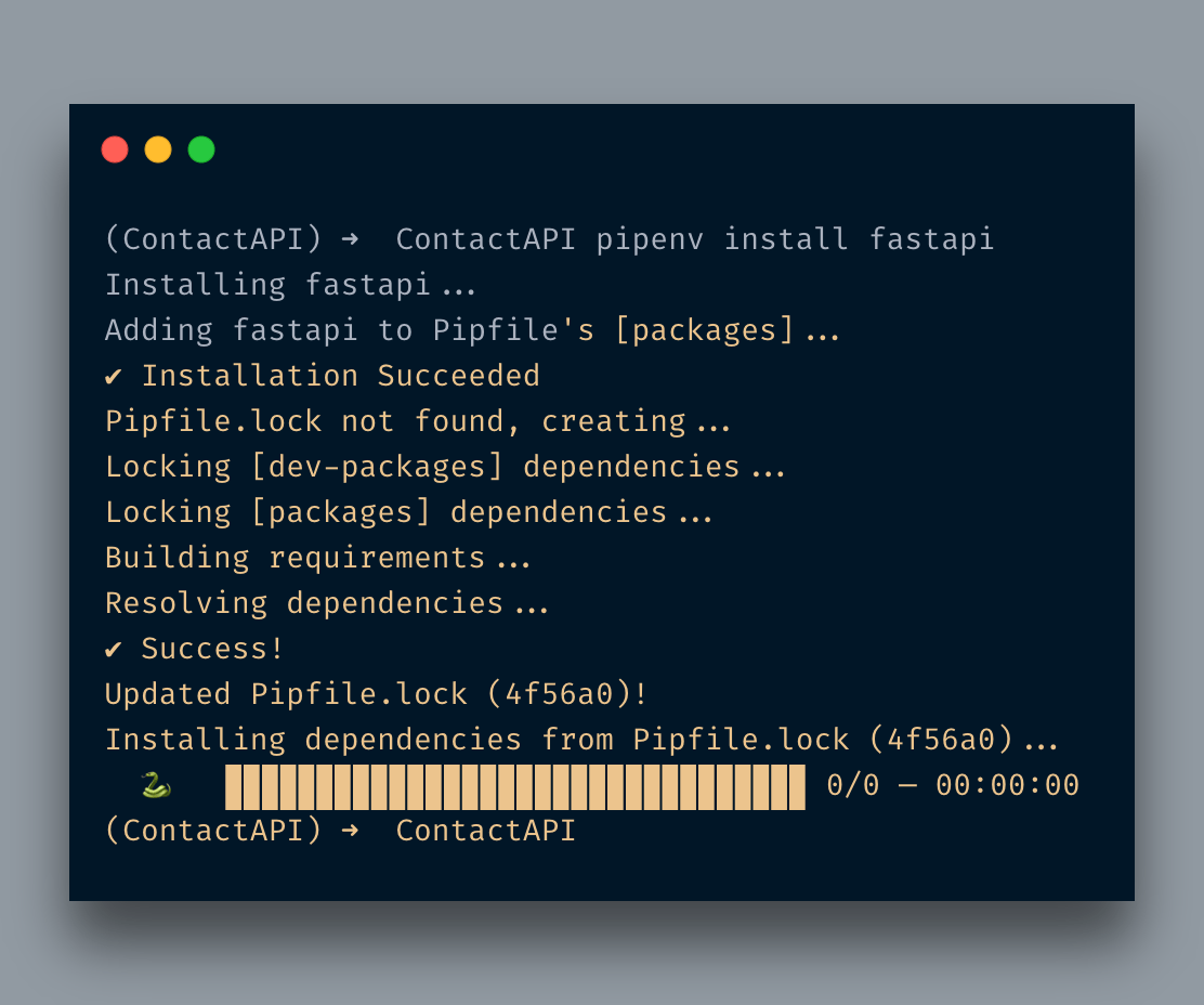
First, we will install FastAPI by running the following command: pipenv install fastapi
Note it’s pipenv, NOT pip. When you are into the shell you will be using pipenv. Underlying it is using pip but all entries are being stored in Pipfile. The Pipfile will be looking like below:
OK, so we have set up our dev environment. It’s time to start writing our first API endpoint. I am going to create a file called main.py. This will be the entry point of our app.
If you have worked on Flask then you will be finding it pretty much similar. After importing the required library you created an app instance and created your first route with a decorator.
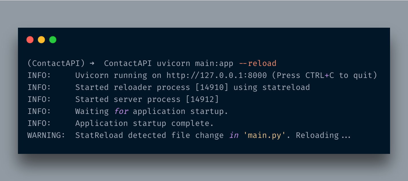
Now you wonder how to run it. Well, FastAPI comes with the uvicorn which is an ASGI server. You will simply be running the command uvicorn main:app --reload
You provide the file name(main.py in this case) and the class object(app in this case) and it will initiate the server. I am using the --reload flag so that it reloads itself after every change.
Visit http://localhost:8000/ and you will see the message in JSON format {"Hello":"FastAPI"}
Cool, No?
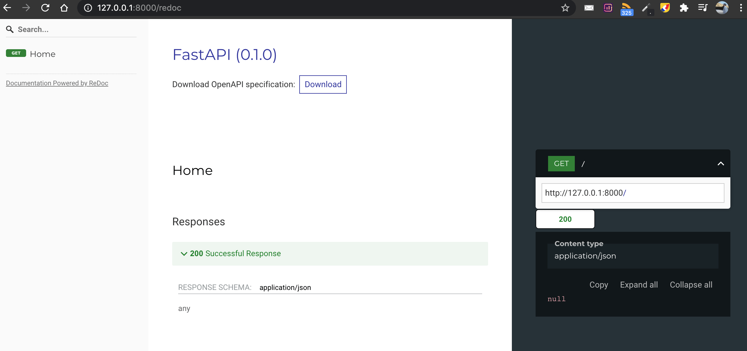
FastAPI provides an API document engine too. If you visit http://localhost:8000/docs which is using the Swagger UI interface.
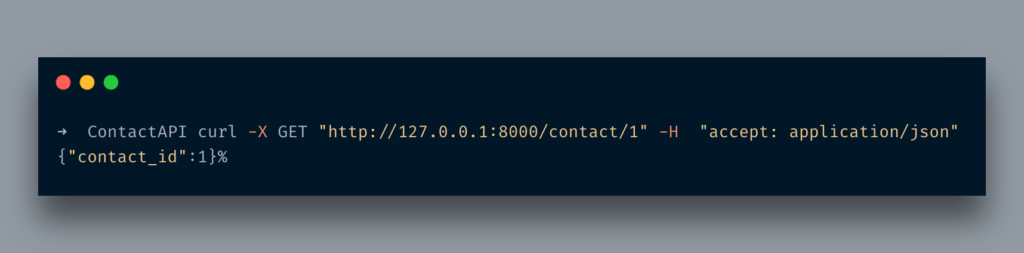
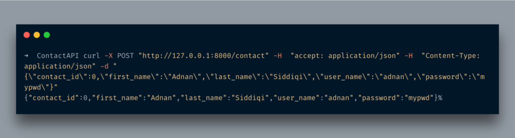
So here is a method, contact_details that accepts only an int parameter and just returns it as it in a dict format. Now when I access it via cURL it looks like below:
Now, what if I pass a string instead of an integer? You will see the below
Did you see it? it returned an error message that you sent the wrong data type. You do not need to write a validator for such petty things. That’s the beauty while working in FaastAPI.
Query String
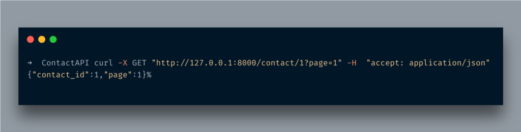
What if you pass extra data in the form of query strings? For instance your API end-point returns loads of records hence you need pagination. Well, no issue, you can fetch that info as well.
Here, I passed another parameter, page and set its type Optional[int] here. Optional, well as the name suggests it’s an optional parameter. Setting the type int is making sure that it only accepts the integer value otherwise, it’d be throwing an error like it did above.
Access the URL http://127.0.0.1:8000/contact/1?page=5 and you will see something like below:
Cool, No?
So far we just manually returned the dict. It is not cool. It is quite common that you input a single value and return a YUUGE JSON structure. FastAPI provides an elegant way to deal with it, using Pydantic models.
Pydantic models actually help in data validation, what does it mean? It means it makes sure that the data which is being passed is valid, if not otherwise it returns an error. We are already using Python’s type hinting and these data models make that the sanitized data is being passed thru. Let’s write a bit of code. I am again going to extend the contact API for this purpose.
I imported the BaseModel class from pydantic. After that, I created a model class that extended the BaseModel class and set 3 fields in it. Do notice I am also setting the type of it. Once it’s done I created a POST API endpoint and passed an Contact parameter to it. I am also using async here which converts the simple python function into a coroutine. FastAPI supports it out of the box.
Go to http://localhost:8080/docs and you will see something like below:
When you run the CURL command you would see something like the below:
As expected it just returned the Contact object in JSON format.
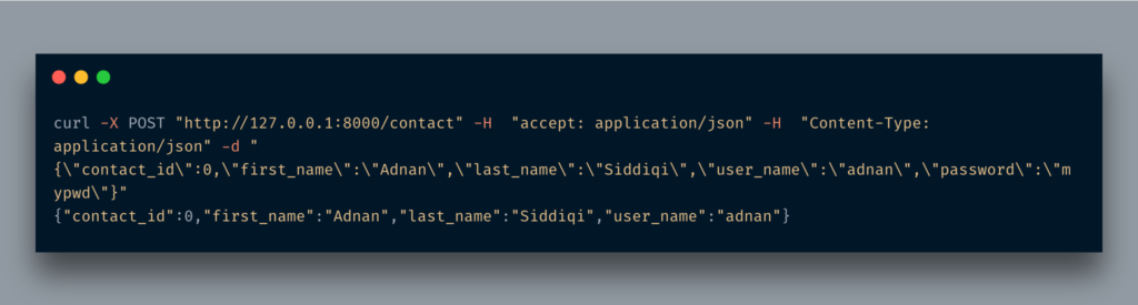
As you notice, it just dumps the entire model in JSON format, including password. It does not make sense even if your password is not in plain-text format. So what to do? Response Model is the answer.
What is Response Model
As the name suggests, a Response Model is a model that is used while sending a response against a request. Basically, when you just used a model it just returns all fields. By using a response model you can control what kind of data should be returned back to the user. Let’s change the code a bit.
I have added another class, ContactOut which is almost a copy of the Contact class. The only thing which is different here is the absence of the password field. In order to use it, we are going to assign it in the response_model parameter of the post decorator. That’s it. Now when I run hit the same URL it will not return the password field.
As you can see, no password field is visible here. If you notice the /docs URL you will see it visible over there as well.
Using a different Response Model is feasible if you are willing to use it in multiple methods but if you just want to omit the confidential information from a single method then you can also use response_model_exclude parameter in the decorator.
The output will be similar. You are setting the response_model and response_model_exclude here. The result is the same. You can also attach metadata with your API endpoint.
@app.post('/contact', response_model=Contact, response_model_exclude={"password"},description="Create a single contact")
async def create_contact(contact: Contact):
    return contact
We added the description of this endpoint which you can see in the doc.
FastAPI documentation awesomeness does not end here, it also lets you set the example JSON structure of the model.
It is always possible that you do not get the required info. FastAPI provides HTTPException class to deal with such situations.
@app.get("/contact/{id}", response_model=Contact, response_model_exclude={"password"},description="Fetch a single contact")
async def contact_details(id: int):
    if id < 1:
        raise HTTPException(status_code=404, detail="The required contact details not found")
    contact = Contact(contact_id=id, first_name='Adnan', last_name='Siddiqi', user_name='adnan1', password='adn34')
    return contact
A simple endpoint. It returns contact details based on the id. If the id is less than 1 it returns a 404 error message with details.
Before I leave, let me tell you how you can send custom headers.
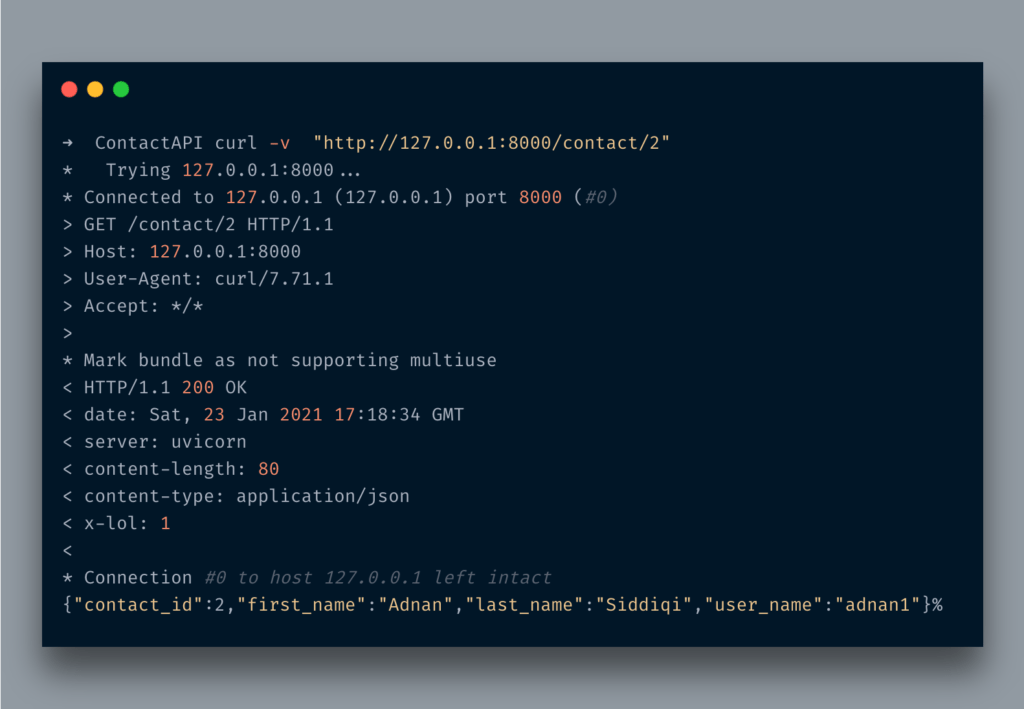
from fastapi import FastAPI, HTTPException, Response@app.get("/contact/{id}", response_model=Contact, response_model_exclude={"password"},
         description="Fetch a single contact")
async def contact_details(id: int, response: Response):
    response.headers["X-LOL"] = "1"
    if id < 1:
        raise HTTPException(status_code=404, detail="The required contact details not found")
    contact = Contact(contact_id=id, first_name='Adnan', last_name='Siddiqi', user_name='adnan1', password='adn34')
    return contact
After importing the Response class I passed request parameter of type Request and set the header X-LOL
After running the curl command you will see something like the below:
You can find x-lol among headers. LOL!
Conclusion
So in this post, you learned how you can start using FastAPI for building high-performance APIs. We already have a minimal framework called Flask but FastAPI’s asynchronous support makes it much attractive for modern production systems especially machine learning models that are accessed via REST APIs. I have only scratched the surface of it. You can learn further about it on the official FastAPI website.
Hopefully, in the next post, I will be discussing some advanced topics like integrating with DB, Authentication, and other things.
As recently as May 2019 Facebook open-sourced some of their recommendation approaches and introduced the DLRM (Deep-learning Recommendation Model). This blog post is meant to explain how and why DLRM and other modern recommendation approaches work so well by looking at how they can be derived from previous results in the domain and by explaining their inner workings and intuitions in detail.
Personalized AI-based advertisement isthe name of the game in online marketing these days and companies like Facebook, Google, Amazon, Netflix, and co are kings of the online marketing jungle because they have not only adopted this trend but have essentially invented it and built their entire business strategies around it. Netflix’s “other movies you might enjoy” or Amazon’s “Customers who bought this item also bought…” are just some examples of many in the online world.
So naturally, the everyday Facebook and Gooogle user that I am, I asked myself at some point:
“HOW EXACTLY DOES THIS THING WORK?“
And yeah, we all know the basic movie recommendation example to explain how collaborative filtering/matrix factorization works. Also, I am not talking about the approach of training a straight-forward classifier per user, that outputs a probability of whether or not that user likes a certain product. Those two approaches, namely collaborative filtering and content-based recommendation have to yield some sort of performance and some predictions that can be used, but Google, Facebook, and co surely must have something better up their sleeves, otherwise they wouldn’t be where they are today.
In order to understand where today’s high-end recommendation systems come from, we have to take a look at two of the basic approaches to the problem of
predicting how much a certain user likes a certain item.
which in the online-marketing world adds up to predicting click-through rates (CTR) for possible ads, based on explicit feedback such as ratings, likes, etc. as well as implicit feedback, such as clicks, search histories, comments, or website visits.
Content-based filtering vs. Collaborative-filtering
1. Content-based filtering
Loosely speaking content-based recommendation means to predict whether a user likes a certain product by using the user’s online history. That includes, among others, likes the user gave (e.g. on Facebook), keywords he/she searched for (e.g. on Google), and simply clicks and visits he/she made to certain websites. All in all, it focuses on the user’s own preferences. We can for example think of a simple binary classifier (or regressor) that outputs a click-through rate (or rating) for a certain ad-group for this user.
2. Collaborative-filtering
Collaborative filtering however tries to predict whether a user might like a certain product by looking at the preferences of similar users. Here we can think of the standard matrix factorization (MF) approach for movie recommendations where the ratings matrix get’s factorized into one embedding matrix for the users and one for the movies.
A disadvantage of classic MF is that we cannot use any side features e.g. movie genre, release date, etc., the MF itself has to learn them from the existing interactions. Also, MF suffers from the so-called “cold start problem”, meaning a new movie that hasn’t been rated by anyone yet, cannot be recommended. Content-based filtering solves these two issues, however, is lacking the predictive power of looking at similar users’ preferences.
The advantages and disadvantages of the two different approaches bring up very clearly the need for a hybrid approach where both ideas are somehow combined into one model.
Hybrid recommendation models
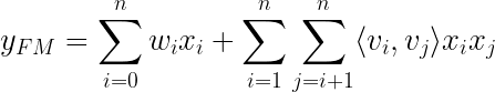
1. Factorization Machine
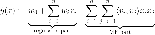
One idea that was introduced by Steffen Rendle in 2010 is the Factorization Machine. It holds the basic mathematical approach to combining matrix factorization with regression
where the model parameters that need to be estimated during learning are:
and ⟨ ∙ , ∙ ⟩ is the dot product between two vectors vᵢ and vⱼof size ℝᵏ, who can be seen as rows in V.
It is pretty straight-forward to see how this equation makes sense when looking at an example of how to represent the data x that gets thrown into this model. Let’s have a look at the described example in the paper on Factorization Machines by Steffen Rendle:
Imagine having the following transaction data on movie reviews where users give ratings to movies at a certain time:
user u ∈ U = {Alice (A), Bob (B), . . .}
movie (item) i ∈ I = {Titanic (TI), Notting Hill (NH), Star Wars (SW), Star Trek (ST), . . .}
rating r ∈ {1,2,3,4,5} at time t ∈ ℝ
Fig.1, S. Rendle — 2010 IEEE International Conference on Data Mining, 2010- “Factorization Machines”
Looking at the figure above we can see the data setup for a hybrid recommendation model. Both the sparse features that represent the user and the item as well as any additional meta or side information (e.g. “Time” or “Last Movie Rated” in this example) are part of a feature vector x that gets mapped to a target y. Now the key is how they are processed by the model.
The regression part of the FM handles both the sparse data (e.g. “User”) as well as the dense data (e.g. “Time”) like a standard regression task and thus can be interpreted as the content-based filtering approach within the FM.
The MF part of the FM now accounts for the interactions between feature blocks (e.g. interaction between “User” and “Movie”), where the matrix V can be interpreted as the embedding matrix used in collaborative filtering approaches. These cross-user-movie relationships, bring us insights such as:
user i who has a similar embedding vᵢ (representing his preferences for movie attributes) as another user j with embedding vⱼ, might very well like similar movies as user j.
Adding the two predictions of the regression part and the MF part together and learning their parameters simultaneously in one cost function leads to the hybrid FM model that now uses a “best of both worlds” approach to making a recommendation for a user.
This hybrid approach of a Factorization Machine at first glance already seems to be a perfect “best of both worlds” model, however, as many different AI fields like NLP or computer vision have proven in the past:
“Throw it in a Neural Net and you will make it even better”
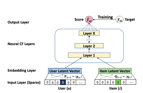
2. Wide and Deep, Neural Collaborative Filtering (NCF) and Deep Factorization Machines (DeepFM)
We will first have a look at how collaborative filtering can be solved by a neural net approach by looking at the NCF paper, this will lead us to Deep Factorization Machines (DeepFM) which are a neural net version of factorization machines. We will see why they are superior to regular FMs and how we can interpret the neural net architecture. We will see how DeepFM was developed as an improvement to the previously released Wide&Deep model by Google, which is one of the first major breakthroughs of deep learning in recommendation systems. This will finally lead us to the aforementioned DLRM paper, released by Facebook in 2019, that can be seen as a simplification and slight adjustment to DeepFM.
NCF
In 2017 a group of researchers released their work on Neural Collaborative Filtering. It contains a generalized framework for learning the functional relationship modeled by matrix factorization in collaborative filtering with a neural network. The authors also explained how to achieve higher-order interactions (MF is only order 2) and how to fuse the two approaches together.
The general idea is that a neural network can (in theory) learn any functional relationship. That means that also the relationship a collaborative filtering model expresses with it’s MF can be learned by a neural net. NCF proposes a simple embedding layer for both users and items (similar to standard MF) followed by a straight-forward multi-layer perceptron neural net to basically learn the MF dot product relationship between the two embeddings via neural net.
Fig.2 from “Neural Collaborative Filtering” by X He, L Liao, H Zhang, L Nie, X Hu, TS Chua — Proceedings of the 26th international conference on world wide web, 2017
The advantage of this approach lies in the non-linearity of the MLP. The simple dot product used in MF will always limit the model to learning interactions of degree 2, whereas a neural net with X layers can in theory learn interactions of a much higher degree. Think of 3 categorical features that all have an interaction, like male, teenager, and RPG computer games for example.
In real-world problems, we don’t just use a user and an item binarized vector as raw input to our embeddings but obviously include various other meta or side information that might be valuable (e.g. age, country, audio/text recordings, timestamp, …) so in reality we have a very high-dimensional, highly sparse and continuous-categorical mixed dataset. At this point, the above presented neural net from Fig. 2 could very well also be interpreted as a content-based recommendation in the form of a simple binary classification feed-forward neural net. And this interpretation is key to understanding how it ends up being a hybrid approach between CF and content-based recommendation. The network can in fact learn any functional relationship, thus interactions in the CF sense of degree 3 or higher, e.g. x₁ ∙ x₂ ∙ x₃, or any non-linear transformation in the classical neural net classification sense of the form σ( … σ(w₁x₁+w₂x₂ + w₃x₃ + b)) can be learned here.
Equipped with the power of learning high-order interactions, we can specifically make it easy for our model to learn also the low order interactions of order 1 and 2, by combining the neural net with a model that is well known to learn low-order interactions, the Factorization Machine. That’s exactly what the authors of DeepFM proposed in their paper. This combination idea, to simultaneously learn high and low-order feature interactions, is the key part of many modern recommender systems and can be found in some form or another in almost every network architecture proposed in the industry.
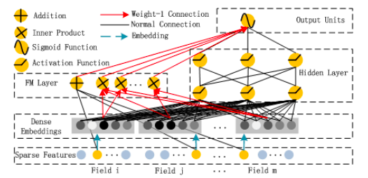
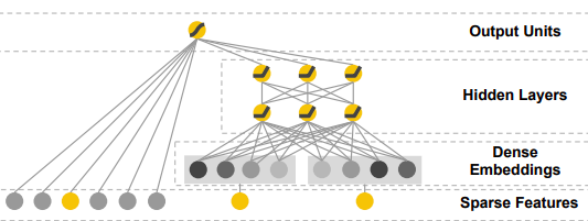
DeepFM
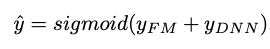
DeepFM is a mixed approach between FM and a deep neural network, that both share the same input embedding layer. Raw features are transformed such that continuous fields are represented by themselves and categorical fields are one-hot encoded. The final (e.g. CTR) prediction, given by the last layer in the NN is defined as:
which is a sigmoid activated sum of the two network components: the FM component and the Deep component.
The FM component is a regular Factorization Machine dressed up in neural net architecture style:
Fig.2 from Huifeng Guo, Ruiming Tang, Yunming Ye, Zhenguo Li, and Xiuqiang He. DeepFM: a factorization machine based neural network for CTR prediction. arXiv preprint arXiv:1703.04247, 2017.
The Addition part of the FM Layer gets the raw input vector x directly (Sparse Features Layer) and multiplies each element with its weight (“Normal Connection”) before summing them up. The Inner Product part of the FM Layer also gets the raw inputs x, but only after they have been passed through the embedding layer and simply takes the dot product without any weight (“Weight-1 Connection”) between the embedding vectors. Adding the two parts together through another “Weight-1 Connection” yields the aforementioned FM equation:
The xᵢxⱼ multiplication in this equation is only needed to be able to write the sum over i=1 through n. It isn’t really part of the neural network computation. The network automatically knows which embedding vectors vᵢ, vⱼ to take the dot product between due to the embedding layer architecture.
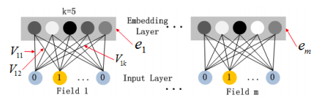
This embedding layer architecture looks as follows:
Fig.4 from Huifeng Guo, Ruiming Tang, Yunming Ye, Zhenguo Li, and Xiuqiang He. DeepFM: a factorization machine based neural network for CTR prediction. arXiv preprint arXiv:1703.04247, 2017.
with Vᵖ being the embedding matrix for each field p={1,…,m} with k columns and however many rows the binarized version of the field has elements. The output of the embedding layer is thus given as:
and it is important to note that this is not a fully connected layer, namely there is no connection between any field’s raw inputs and any other field’s embedding. Think of it this way: the one-hot encoded vector for gender (e.g. (0,1)) cannot have anything to do with the embedding vector for weekday (e.g. (0,1,0,0,0,0,0) raw binarized weekday “Tuesday” and it’s embedding vector with e.g.: k=4; (12,4,5,9)).
The FM component being a Factorization Machine reflects the high importance of both order 1 and order 2 interactions, which are directly added to the Deep component output and fed into the sigmoid activation in the final layer.
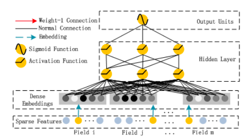
The Deep Component is proposed to be any deep neural net architecture in theory. The authors specifically took a look at a regular feed-forward MLP neural net (as well as a so-called PNN). The regular MLP is given by the following figure:
Fig.3 from Huifeng Guo, Ruiming Tang, Yunming Ye, Zhenguo Li, and Xiuqiang He. DeepFM: a factorization machine based neural network for CTR prediction. arXiv preprint arXiv:1703.04247, 2017.
a standard MLP network with embedding layer between the raw data (highly sparse due to one-hot-encoded categorical input) and the following neural net layers given as:
with σ the activation function, W the weight matrix, a the activation from the previous layer, and b the bias.
This yields the overall DeepFM network architecture:
with the parameters:
latent vector Vᵢ to measure impact of feature i’s interactions with other features (Embedding layer)
Vᵢ gets passed to the FM component to model order-2 interactions (FM Component)
wᵢ weighting the order 1 importance of raw feature i (FM Component)
Vᵢ also gets passed to the Deep component to model all higher-order interactions (>2) (Deep Component)
Wˡ and bˡ, the neural net’s weights and biasses (Deep Component)
The key to getting both high and low order interactions simultaneously is training all parameters at the same time under one cost function, specifically using the same embedding layer for both the FM as well as the Deep component.
Comparison to Wide&Deep and NeuMF
There are many variations that one can dream up on how to tweak this architecture to potentially make it even better. At the core, however, they are all similar in their hybrid approach on how to model high and low order interactions simultaneously. The authors of DeepFM also proposed interchanging the MLP part with a so-called PNN, a deep neural network that gets the FM layer as initial input combined with the embedding layer
The authors of the NCF paper also came up with a similar architecture which they called NeuMF (“Neural Matrix Factorization”). Instead of having an FM as low-order component, they used a regular matrix factorization fed into an activation function. This approach however is lacking the specific order 1 interactions modeled by the linear part of the FM. Also, the authors specifically allowed the model to learn different user and item embeddings for the matrix factorization as well as the MLP part.
As mentioned before, Google’s research team was one of the first to propose a neural network for a hybrid recommendation approach. DeepFM can be thought of as a further development of Google’s Wide&Deep algorithm that looks like this:
Fig.1 from Heng-Tze Cheng, Levent Koc, Jeremiah Harmsen, Tal Shaked, Tushar Chandra, Hrishi Aradhye, Glen Anderson, Greg Corrado, Wei Chai, Mustafa Ispir, Rohan Anil, Zakaria Haque, Lichan Hong, Vihan Jain, Xiaobing Liu, and Hemal Shah. Wide & deep learning for recommender systems. In Proc. 1st Workshop on Deep Learning for Recommender Systems, pages 7–10, 2016.
The right side is our well-known MLP with an embedding layer, the left side however has different, manually engineered, inputs that are directly fed into the final overall output unit. The low-order interaction in the form of the dot product operation is hidden in these manually engineered features, that the authors say can be many different things, for example:
which captures the interactions between d features (with or without another previous embedding) by cross multiplying them (exponent equals 1 if xᵢ is part of k-th transformation) with each other.
It is easy to see how DeepFM is an improvement since it does not require any a priori feature engineering and is able to learn low and high-order interactions from exactly the same input data that all share one common embedding layer. DeepFM really has the FM model as part of its core network, whereas Wide&Deep does not do dot product computations as part of the actual neural net but beforehand in feature engineering steps.
3. DLRM — Deep Learning Recommendation Model
So with all these different options from Google, Huawei (research team around the DeepFM architecture), and others, let’s take a look at how Facebook views things. They came out with their DLRM paper in 2019, which focuses a lot on the practical side of these models. Parallel training setup, GPU computing as well as different handling of continuous vs categorical features.
The DLRM architecture is described in the below figure and works as follows: Categorical features are each represented by an embedding vector, while continuous features are processed by an MLP such that they have the same length as the embedding vectors. Now in a second stage, the dot product between all combinations of embedding vectors and processed (MLP output) dense vectors is computed. Afterward, the dot products are concatenated with the MLP output of the dense features and passed through another MLP and finally into a sigmoid function to give a probability.
DLRM Network as described by DLRM. Figure by Max Beckers.
This DLRM proposal is somewhat of a simplified and modified version of DeepFM in the sense that it also uses dot product computations between embedding vectors but it specifically tries to stay away from high-order interactions by not directly forcing the embedded categorical features through an MLP layer. The design is tailored to mimic the way Factorization Machines compute the second-order interactions between the embeddings. We can think of the entire DLRM setup as the specialized part of DeepFM, the FM component. The classical Deep Component of DeepFM that gets added to the outcome of the FM component in the final layer of DeepFM (and then fed into a sigmoid function) can be seen as completely omitted in the DLRM setup. The theoretical advantages of DeepFM are clear as it is, by design, better equipped to learn high order interaction, however according to Facebook:
“… higherorder interactions beyond second-order found in other networks may not necessarily be worth the additional computational/memory cost”
4. Outlook and Coding
Having introduced various deep recommendation approaches, their intuitions as well as pros and cons, in theory, I had a look at the proposed PyTorch implementation of DLRM on Facebook’s GitHub page.
I checked out the details of the implementation and tried out the predefined dataset APIs that they have built-in to handle different raw datasets directly. Both the Kaggle display advertising challenge by Criteo as well as their Terabyte dataset are pre implemented and can be downloaded and subsequently used to train a full DLRM with just one bash command (see DLRM repo for instructions). I then extended Facebook’s DLRM model API to include preprocessing and data loading steps for another dataset, the 2020 DIGIX Advertisement CTR Prediction. Please check it out here.
In a similar fashion after downloading and unzipping the digix data you can now train a model on this data with a single bash command as well. All the preprocessing steps, shapes of the embeddings, and neural net architecture parameters are adjusted towards handling the digix dataset. A notebook that takes you through the commands can be found here. The model delivers some decent results, as I am continuing to work on it to improve the performance by understanding the raw data and the advertisement process behind the digix data better. Specific data cleaning, hyperparameter tuning, and feature engineering are all things I would like to further work on and are mentioned in the notebook. The first goal was simply to have a technically sound extension of the DLRM model API that can use the raw digix data as input.
All in all, I believe hybrid deep models are one of the most powerful tools for solving recommendation tasks. However, there have been some seriously interesting and creative unsupervised approaches on solving collaborative filtering problems recently using autoencoders. So at this point, I can only guess what the large internet giants are using today to feed us ads we are most likely to click on. I assume that it very well could be a combo of the aforementioned autoencoder approach as well as some form of the deep hybrid models presented in this article.
References
Steffen Rendle. Factorization machines. In Proc. 2010 IEEE International Conference on Data Mining, pages 995–1000, 2010.
Xiangnan He, Lizi Liao, Hanwang Zhang, Liqiang Nie, Xia Hu, and Tat-Seng Chua. Neural collaborative filtering. In Proc. 26th Int. Conf. World Wide Web, pages 173–182, 2017.
Huifeng Guo, Ruiming Tang, Yunming Ye, Zhenguo Li, and Xiuqiang He. DeepFM: a factorizationmachine based neural network for CTR prediction. arXiv preprint arXiv:1703.04247, 2017.
Jianxun Lian, Xiaohuan Zhou, Fuzheng Zhang, Zhongxia Chen, Xing Xie, and Guangzhong Sun. xDeepFM: Combining explicit and implicit feature interactions for recommender systems. In Proc. of the 24th ACM SIGKDD International Conference on Knowledge Discovery & Data Mining, pages 1754–1763. ACM, 2018.
Heng-Tze Cheng, Levent Koc, Jeremiah Harmsen, Tal Shaked, Tushar Chandra, Hrishi Aradhye, Glen Anderson, Greg Corrado, Wei Chai, Mustafa Ispir, Rohan Anil, Zakaria Haque, Lichan Hong, Vihan Jain, Xiaobing Liu, and Hemal Shah. Wide & deep learning for recommender systems. In Proc. 1st Workshop on Deep Learning for Recommender Systems, pages 7–10, 2016.
M. Naumov, D. Mudigere, H. M. Shi, J. Huang, N. Sundaraman, J. Park, X. Wang, U. Gupta, C. Wu, A. G. Azzolini, D. Dzhulgakov, A. Mallevich, I. Cherniavskii, Y. Lu, R. Krishnamoorthi, A. Yu, V. Kondratenko, S. Pereira, X. Chen, W. Chen, V. Rao, B. Jia, L. Xiong, and M. Smelyanskiy, “Deep learning recommendation model for personalization and recommendation systems,” CoRR, vol. abs/1906.00091, 2019. [Online]. Available: http://arxiv.org/abs/1906. 00091 [39]
This one doesn’t need much introduction. Thousands of articles, papers have been written and a few wars have been fought on Bayesian vs Frequentism. In my experience, most folks start with usual linear regression and work their way up to build more complex models and only a few get to dip their feet in the holy pool of Bayes and this lack of opportunity along with the terseness of the topic punches holes in the understanding, at least for me it did.
I don’t want to bebogged down by too many mathematical equations and want to have an intuitive understanding of what, why, and where of the Bayesian statistics. This is my humble attempt to do so.
Let’s build an intuition for Bayesian analysis. I believe one time or the other you might have been sucked in the debate between Frequentism vs Bayesian. There is a lot of literature out there that can explain the difference between the two approaches of statistical inference.
In short, Frequentism is the usual approach of learning from the data, using p-values to measure the significance of variables. The frequentist approach is about point estimates. If my linear equation is:
y is the response variable, x₁, x₂ are the dependent variables. β₁ and β₂ are the coefficients that need to be estimated. β₀ is the intercept term; If x₁ changes by 1 unit then y is affected by β₁ units e.g. if x₁ is 1 and β₁ is 2 then y will be affected by 2 units. Usual linear stuff. The thing to note here is that the regression equation estimates values of various β, that best explain the data at hand, based on minimising the sum of squared errors(line of best fit) and the estimated values are singular point i.e. there will be one value for β₀, one for β₁, and one for β₂, and so on. The estimated values of β are known as the maximum likelihood estimate of β because it is the value that is the most probable given the inputs, x, and output, y.
Bayesiandiffers from the frequentist approach in the fact that apart from the data, it takes the prior knowledge of the data into account. That’s where the beef lies between the two groups. Frequentists take data as the gospel while Bayesians think there is always something that we know about the system and why not use it in the estimation of the parameters.
The data along with the prior knowledge are taken together to estimate what’s known as the posterior and it is not a single value but a distribution. Bayesian methods estimate a posterior distribution of the model parameters, not a single best value as is the case in the frequentist approach.
The priors that we choose for the model parameters are not single values but they are distributions as well, they could be Normal, Cauchy, Binomial, Beta or any other distribution deemed fit according to our guess.
I hope you are aware of the vernacular and script of Bayes’ theorem
(Feel free to skip this section if you already understand Bayes’s Theorem)
Although, it is quite self-explanatory but let me just explain with the help of a very basic example.
P(A|B) refers to the probability of A given B has already happened. e.g. A random card is drawn from a deck of 52 cards, what is the probability that it is King GIVEN we drew a hearts card?
A = Card is King, B = Card is from Hearts suite.
P(A= King|B = Hearts)
P(A) = P(King) = 4/52 = 1/13
P(B) = P(Hearts) = 13/52 = 1/4
P(B|A) = P(Hearts| King) = Probability of getting a Hearts card GIVEN it is King = 1/4 (There are 4 kings in a set of 52 and you can select only one king of hearts out of those 4 kings)
Putting it all together, P(A|B) = (1/4). (1/13) / (1/4) = 1/13, so there are 1 in 13 chances to get a king given it is hearts.
I chose this simple example because it doesn’t really need Bayes’ rule to solve so even the beginners can think about it intuitively; Given it is a hearts’ card, the probability of getting a king is 1 out of 13.
How does the Bayesian approach include prior information?
P(A) is the value that we have approximated or what we have data on. In the above example, P(A) is the probability of getting a king irrespective of the suite. We know that the probability of getting a king is 1/4, so instead of starting with a clean slate, we are providing a value of 0.25 to the system.
By the way, Thomas Bayes didn’t come up with the above equation Laplace did. Bayes wrote a paper “An Essay towards solving a Problem in the Doctrine of Chances” on his thought experiments. After Bayes’ death, his friend Richard Price found the paper and after a few editions by him, the paper was read at the Royal Society of London.
For the Bayesian inference:
P(β|y, X) is the called the posterior distribution of the model parameters, β, given the data X and y, where X is input and y is output.
P(y|β, X) is the likelihood of the data which is multiplied by the prior probability of the parameters, P(β|X), and divided by P(y|X) which is known as a normalization constant. This normalisation parameter is required to make the sum of values in P(β|y, X) equals 1.
In nutshell, we are using our prior information about the model parameters and the data to estimate posterior.
Give yourself a pat on the back if you have made it this far! 🙂
Source: Giphy.com
A lot of Bayesian aligned thinkers attribute the solution of Enigma to Alan Turing. Well, yes, he did indeed build the probabilistic model but Polish Mathematicians helped him. Long before the war, Polish mathematicians had solved the enigma using Mathematical approach when Britishers were still trying to solve it linguistically. Hail Marian Rejewski!
Moment of truth through an example
Let’s see if we can understand what we learned above with some simple example to build our intuition.
Let’s toss a coin 20 times, 1 is heads and 0 is tails. Here are the outcomes of the coin throws:
The mean of this data is 0.75; in other words, there are 75% chances of getting heads i.e. 1 rather than getting a tail i.e. 0
By the way, any process that has canonically only two outcomes 0 or 1is referred to as Bernoulli process.
Taking a frequentist approach, it seems the coin is biased i.e. if we toss it one more time then according to frequentist estimates, it is more likely (75% of the times)that the coin will turn up heads i.e.1.
Although, most coins aren’t biased and the probability of getting a 1 or a 0 should be 50%. According to the central limit theorem, if we had tossed the coin infinite times then the probabilities would have lined up to be 0.5 for both head and tails. Real-life is quite different from theorems, no one is going to toss a coin infinite times; we have to make decisions on whatever data is available to us.
That’s where the Bayesian approach is helpful. It gives us the freedom to include the priors(our initial beliefs) and that’s what we will do to the coin flip data. If we don’t have any information about the priors then we can use a completely uninformative uniform distribution — in practice, the results of the uniform distribution will be same as the frequentist approach because we are telling our model that each possibility is equally likely.
Non-Bayesian(Frequentist) = Bayesian with a uniform prior
Uninformative prior gives the same results as the frequentist approach(Image by Author)
In the chart above, posterior and frequentist results coincide and it peaks at around 0.75( just like the frequentist approach). Prior is a straight line because we assumed that a uniform distribution. In this case, the green distribution is actually a likelihood.
I believe we can do better than that. Let’s change our prior to something more informed, maybe a beta distribution and observe the results.
Prior changed to a beta distribution and we see that it is doing better than frequentist(Image by Author)
This seems better. Our prior has changed and because of that the posterior has moved towards the left, it isn’t near the 0.5 value but it isn’t at least coincidental with the frequentist at 0.75.
We can improve it further by tweaking a few params of our prior distribution so that it becomes more opinionated.
An opinionated prior which makes the results of the Bayesian approach mimick the real world as compared to frequentist(Image by Author)
This seems much better, the posterior has shifted as we have changed our prior and is much more in line with the fact that an unbiased coin will yield heads 50% of the time and tales rest of the time.
Our existing knowledge about the coin had a major impact on the results and that makes sense. It is the polar opposite to the frequentist approach in which we assume that we know NOTHING about the coin and these 20 observations are the gospel.
Conclusion
So you see how through Bayesian, despite having a paucity of data, we were able to reach the approximately right conclusion when we included our initial beliefs in the model. Bayes’ rule is behind the intuition of Bayesian statistics(such an obvious statement to make) and it provides an alternative to frequentism.
The Bayesian approach incorporates prior information and that can be a solid tool when we have limited data.
2. The approach seems intuitive — estimate what your solution would be and improve that estimate as you gather more data.
Please understand that it doesn’t mean that Bayesian is the best approach for solving all data science problems; It is only one of the approaches and it would be fruitful to learn both Bayesian and Frequentist methods rather than fighting the crusades between these schools of thoughts.
With great power comes great responsibility. Take everything with a grain of salt. Although there are apparent advantages of Bayesian methods, it is much easier to produce highly biased results. One can choose a prior that can shift the entire results. As an example, it is much easier and cheaper to choose the ‘right’ prior than invest millions of dollars in research and development of safer and effective drugs in the pharmaceutical world. When billions of dollars are on the line, it’s easier to publish mediocre studies in predatory journals and use them as your prior.
Further reading:
Johnson, S. (2002). Emergence: The connected lives of ants, brains, cities, and software. Simon and Schuster.