
 hyungseok
2021년 4월 30일 모바일 게임 매출 순위
| Rank | Game | Publisher |
|---|---|---|
| 1 | 리니지2M | NCSOFT |
| 2 | 리니지M | NCSOFT |
| 3 | Cookie Run: Kingdom – Kingdom Builder & Battle RPG | Devsisters Corporation |
| 4 | 기적의 검 | 4399 KOREA |
| 5 | 세븐나이츠2 | Netmarble |
| 6 | Genshin Impact | miHoYo Limited |
| 7 | 뮤 아크엔젤 | Webzen Inc. |
| 8 | 라이즈 오브 킹덤즈 | LilithGames |
| 9 | 블레이드&소울 레볼루션 | Netmarble |
| 10 | 그랑사가 | NPIXEL |
| 11 | V4 | NEXON Company |
| 12 | 삼국지 전략판 | Qookka Games |
| 13 | 데카론M | THUMBAGE |
| 14 | 원펀맨: 최강의 남자 | GAMENOW TECHNOLOGY |
| 15 | 바람의나라: 연 | NEXON Company |
| 16 | R2M | Webzen Inc. |
| 17 | 가디언 테일즈 | Kakao Games Corp. |
| 18 | S.O.S: 스테이트 오브 서바이벌 x 더 워킹 데드 | KingsGroup Holdings |
| 19 | Roblox | Roblox Corporation |
| 20 | 리니지2 레볼루션 | Netmarble |
| 21 | 파이널삼국지2 | Gamepub |
| 22 | Brawl Stars | Supercell |
| 23 | AFK 아레나 | LilithGames |
| 24 | PUBG MOBILE | KRAFTON, Inc. |
| 25 | FIFA Mobile | NEXON Company |
| 26 | A3: 스틸얼라이브 | Netmarble |
| 27 | DK모바일: 영웅의귀환 | NTRANCE Corp |
| 28 | Empires & Puzzles: Epic Match 3 | Small Giant Games |
| 29 | 컴투스프로야구2021 | Com2uS |
| 30 | 메이플스토리M | NEXON Company |
| 31 | Lords Mobile: Kingdom Wars | IGG.COM |
| 32 | 조선협객전M | withHUG |
| 33 | 페이트/그랜드 오더 | Netmarble |
| 34 | 붕괴3rd | miHoYo Limited |
| 35 | Summoners War | Com2uS |
| 36 | Top War: Battle Game | Topwar Studio |
| 37 | 미르4 | Wemade Co., Ltd |
| 38 | Gardenscapes | Playrix |
| 39 | Cookie Run: OvenBreak – Endless Running Platformer | Devsisters Corporation |
| 40 | Age of Z Origins | Camel Games Limited |
| 41 | FIFA ONLINE 4 M by EA SPORTS™ | NEXON Company |
| 42 | Pmang Poker : Casino Royal | NEOWIZ corp |
| 43 | 삼국지혼 | YOUZU(SINGAPORE)PTE.LTD. |
| 44 | 이카루스 이터널 | LINE Games |
| 45 | 검은강호2: 이터널 소울 | 9SplayDeveloper |
| 46 | KartRider Rush+ | NEXON Company |
| 47 | 신명2:아수라 | Trigirls Studio |
| 48 | 프로야구 H3 | NCSOFT |
| 49 | Gunship Battle Total Warfare | JOYCITY Corp. |
| 50 | 프린세스 커넥트! Re:Dive | Kakao Games Corp. |
Deep Learning with Keras Cheat Sheet (2021), Python for Data Science -번역
KERAS 치트 시트 (2021), 데이터 과학을위한 파이썬으로 깊은 학습
2021 년에 깊은 학습을위한 초보자를위한 절대적인 기본 사항

Keras는 깊은 학습 모델을 개발하고 평가하기 위해 고급 신경 네트워크 API를 제공하는 Tensorflow를위한 강력하고 사용하기 쉬운 깊은 학습 라이브러리입니다.
KERAS를 최적화하여 다양한 깊은 학습 모델을 만드는 방법을 배우려면 아래 섹션을 확인하십시오.
섹션 :
1.기본 예제
2.데이터
삼.사전 처리
4.모델 아키텍처
5.컴파일 모델
6.모델 훈련
7.예측
8.모델의 성능을 평가하십시오
9.모델을 저장 / 다시로드하십시오
Basic Example
아래 코드는 KERAS를 사용하여 데이터 집합에서 깊은 학습 모델을 만들고 실행하는 기본 단계를 보여줍니다.
코드의 단계는 다음과 같습니다. loadi엔g 데이터를 전처리하고, 모델을 생성하고, 모델에 레이어를 추가하고, 데이터에 모델을 구성하고, 트레이닝 된 모델을 사용하여 테스트 세트에 대한 예측을하고, 마침내 모델의 성능을 평가하는 데이터를
& gt; & gt;numpy를 np로 가져 오기
& gt; & gt;Keras.Models 가져 오기 순차적으로
& gt; & gt;Keras.Layers에서 가져 오기 밀도
& gt; & gt;Keras.Datasets에서 Boston_Housing 가져 오기
& gt; & gt;(x_train, y_train), (x_test, y_test) = boston_housing.load_data ()
& gt; & gt;모델 = 순차 ()
& gt; & gt;model.add (빽빽한 (12, 활성화 = 'RELU', input_dim = 8))
& gt; & gt;model.add (빽빽한 (1))
& gt; & gt;model.compile (Optimizer = 'rmsprop', loss = 'mse', metrics = [ 'ma']))
& gt; & gt;model.fit (x_train, y_train, batch_size = 32, epochs = 15)
& gt; & gt;model.predict (x_test, batch_size = 32)
& gt; & gt;Score = model.evaluate (x_test, y_test, batch_size = 32)
Data
데이터를 숫자 배열로 저장하거나 숫자 배열 목록으로 저장해야합니다.이상적으로는 Sklearn.cross_validation의 train_test_split 모듈에도 해당하는 교육 및 테스트 세트의 데이터를 분리합니다.
예제 데이터 집합의 경우 Keras 라이브러리에 통합 된 Boson Housing DataSet을 사용할 수 있습니다.
& gt; & gt;Keras.Datasets에서 Boston_Housing 가져 오기
& gt; & gt;(x_train, y_train), (x_test, y_test) = boston_housing.load_data ()
Preprocessing
데이터 집합을 가져온 후 모델이 적합 할 준비가되지 않을 수 있습니다.이 경우 모델에 대한 데이터를 준비하기 위해 사전 처리를해야합니다.
범주 구성 기능 인코딩
0과 n_classes-1 사이의 값을 가진 대상 레이블을 인코딩합니다.
& gt; & gt;keras.utils 가져 오기 to_categorical.
& gt; & gt;y_train = to_categorical (y_train, num_classes)
& gt; & gt;y_test = to_categorical (y_test, num_classes)
Train and Test Sets
데이터 세트를 X 및 Y 변수 모두에 대한 교육 및 테스트 세트로 분할합니다.
& gt; & gt;SKLEARN.MODEL_SELECTION IMPORT TRAT_TEST_SPLIT.
& gt; & gt;x_train, x_test, y_train, y_test = train_test_split (x, y,
test_size = 0.33, random_state = 42)
Standardization
표준화는 평균 및 확장을 단위 분산으로 제거하여 기능입니다.
& gt; & gt;SKLEARN.PREPROPESSING 가져 오기 StandardScaler에서
& gt; & gt;스케일러 = StandardScaler (). 맞춤 (x_train)
& gt; & gt;Standardized_x = scaler.transform (x_train)
& gt; & gt;표준화 된 _x_test = scaler.transform (x_test)
Model Architecture
이 섹션에서는 레이어별로 다른 깊은 학습 모델 레이어를 구축하는 방법을 배우게됩니다.
순차 모델
순차적 인 모델은 각 층이 정확히 하나의 입력 텐서 및 하나의 출력 텐서를 갖는 평평한 층의 일반 스택에 적합합니다.이것은 일반적으로 어떤 모델에서도 추가 할 첫 번째 레이어입니다.
& gt; & gt;Keras.Models 가져 오기 순차적으로
& gt; & gt;모델 = 순차 ()
Artificial Neural Network (ANN)
깊은 학습 모델을 위해 사용되었습니다분류과회귀.
바이너리 분류 :
아래 코드는 바이너리 분류에 사용되는 ANN 모델의 예입니다 (0 또는 1로 클래스를 식별하십시오).코드는 모델에 3 개의 계층을 추가합니다.첫 번째는 입력 레이어이며 12 개의 노드가 있으며, 제 2 계층은 8 개의 노드를 가지며, 마지막 층은 출력 노드 또는 예측 된 것인 것입니다.
& gt; & gt;Keras.Layers에서 가져 오기 밀도
& gt; & gt;model.add (짙은 (12, input_dim = 8, kernel_initializer = '유니폼',
활성화 = 'RELU')))
& gt; & gt;model.add (빽빽한 (8, kernel_initializer = 'uniform', 활성화 = 'RELU'))
& gt; & gt;model.add (짙은 (1, kernel_initializer = 'uniform', 활성화 = 'sigmoid'))
멀티 클래스 분류 :
아래 코드는 다중 클래스 분류에 사용되는 앤 모델의 예입니다.코드는 모델에 4 개의 레이어를 추가합니다.첫 번째는 입력 레이어이며 52 개의 노드가 있으며, 두 번째는 오버 퍼팅을 줄이는 데 사용되는 드롭 아웃 층이며, 제 3 계층은 52 개의 노드를 가지며, 마지막 층은 특정 관찰이 10 가지 중 하나로 이동하는 확률 인 10 개의 노드를 가지고 있습니다.클래스.
& gt; & gt;Keras.Layers 가져 오기 드롭 아웃
& gt; & gt;model.add (조밀 한 (52, 활성화 = 'RELU'), input_shape = (78,))
& gt; & gt;model.add (드롭 아웃 (0.2))
& gt; & gt;model.add (빽빽한 (52, 활성화 = 'RELU'))
& gt; & gt;model.add (짙은 (10, 활성화 = 'softmax'))
회귀 :
아래 코드는 회귀에 사용되는 앤 모델의 예입니다.코드는 모델에 2 개의 레이어를 추가합니다.첫 번째는 64 개의 노드를 갖는 입력 계층이고, 제 2는 예측 된 값인 단지 1 개의 노드를 갖는 출력 계층이다.
& gt; & gt;model.add (조밀함 (64, 활성화 = 'RELU', input_dim = train_data.shape [1]))
& gt; & gt;
model.add (빽빽한 (1))
Convolution Neural Network (CNN)
깊은 학습 모델그림의 분류.이 모델은 상당히 복잡하며 아래 코드에서 볼 수있는 꽤 많은 레이어가 포함되어 있습니다.그 코드는 CNN 모델이 보이는 것의 기본 예를 제공합니다.
각 계층이 무엇을 확인하는지 이해하고 싶다면Keras 문서.
>>> from keras.layers import Activation,Conv2D,MaxPooling2D,Flatten >>> model2.add(Conv2D(32,(3,3),padding='same',input_shape=x_train.shape[1:]))
>>> model2.add(Activation('relu'))
>>> model2.add(Conv2D(32,(3,3)))
>>> model2.add(Activation('relu'))
>>> model2.add(MaxPooling2D(pool_size=(2,2)))
>>> model2.add(Dropout(0.25))
>>> model2.add(Conv2D(64,(3,3), padding='same'))
>>> model2.add(Activation('relu'))
>>> model2.add(Conv2D(64,(3, 3)))
>>> model2.add(Activation('relu'))
>>> model2.add(MaxPooling2D(pool_size=(2,2)))
>>> model2.add(Dropout(0.25))
>>> model2.add(Flatten())
>>> model2.add(Dense(512))
>>> model2.add(Activation('relu'))
>>> model2.add(Dropout(0.5))
>>> model2.add(Dense(num_classes))
>>> model2.add(Activation('softmax'))
Recurrent Neural Network (RNN)
깊은 학습 모델시간 시리즈.
아래 코드는 시계열에 사용되는 RNN 모델의 예입니다.코드는 모델에 3 개의 계층을 추가합니다.첫 번째 레이어는 입력 레이어이고, 두 번째 레이어는 긴 단기 메모리라고 불리는 것이며 세 번째 레이어는 출력 레이어이거나 모델에서 예측 된 것입니다.
& gt; & gt;keras.klayers 수입 embedding, lstm.
& gt; & gt;model.add (Empedding (20000,128))
& gt; & gt;model.add (lstm (128, dropout = 0.2, recurrent_dropout = 0.2))
& gt; & gt;model.add (빽빽한 (1, 활성화 = 'sigmoid'))
Compile Model
모델이 구성된 후에는 모델을 컴파일합니다.컴파일하면 모델을 훈련하고 평가하는 데 사용될 교육 구성 (최적화, 손실, 메트릭)을 사용하려는 작업을 지정합니다.
Ann : 바이너리 분류
바이너리 분류에 사용되는 Ann 모델에 대해 이러한 교육 구성을 사용하십시오.
& gt; & gt;model.compile (Optimizer = 'Adam',
손실 = 'binary_crossentropy',
메트릭 = [ '정확도'])
ANN: Multi-Class Classification
멀티 클래스 분류에 사용되는 앤 모델에 대해 이러한 교육 구성을 사용하십시오.
& gt; & gt;model.compile (Optimizer = 'rmsprop',
손실 = 'categorical_crossentropy',
메트릭 = [ '정확도'])
ANN: Regression
회귀 분석에 사용되는 앤 모델에 대해 이러한 교육 구성을 사용하십시오.
& gt; & gt;model.compile (Optimizer = 'rmsprop',
손실 = 'MSE',
메트릭 = [ 'mae'])
Recurrent Neural Network
RNN 모델에 대해 이러한 교육 구성을 사용하십시오.
& gt; & gt;model.compile (loss = 'binary_crossentropy',
Optimizer = 'Adam',
메트릭 = [ '정확도'])
Model Training
모델을 컴파일 한 후에는 이제 교육 세트에 맞게 맞게됩니다.배치 크기는 한 번에 모델에 얼마나 많은 관찰을 입력하는지 결정하고 epochs는 모델이 교육 세트에 맞게 원하는 횟수를 나타냅니다.
& gt; & gt;model.fit (x_train,
Y_Train,
batch_size = 32,
epochs = 15)
Prediction
숙련 된 모델을 사용하여 테스트 세트를 예측합니다
& gt; & gt;model.predict (x_test, batch_size = 32)
Evaluate Your Model’s Performace
테스트 세트에서 모델이 얼마나 잘 수행되는지 결정하십시오.
& gt; & gt;Score = model.evaluate (x_test, y_test, batch_size = 32)
Save/Reload Models
깊은 학습 모델은 훈련하고 실행하는 데 꽤 오랜 시간이 걸릴 수 있으므로 완료되면 다시 저장하고 다시로드 할 수 있으므로 해당 프로세스를 통과 할 필요가 없습니다.
& gt; & gt;keras.models 가져 오기 load_model.
& gt; & gt;model.save ( 'model_file.h5')
& gt; & gt;my_model = load_model ( 'my_model.h5')
Python은 현재 및 가까운 장래에 데이터 과학에 관해서 상위 개입니다.깊은 학습을위한 가장 강력한 라이브러리 중 하나 인 Keras에 대한 지식은 종종 오늘날 데이터 과학자들에게 요구 사항입니다.
이 치트 시트를 처음에 가이드로 사용하고 필요할 때 다시 돌아 오면 Keras Library를 마스터하는 방법에 잘 될 것입니다.
Keras 라이브러리와 함수에 대해 더 자세히 알고 싶다면 설명서를 확인하지 않았습니다.keras.,여전히 많은 유용한 기능이 있으므로 배워야합니다.
2K + 사람들이있는 내 이메일 목록에 가입하여 데이터 과학 치트 시트 소책자가 무료로 완전한 파이썬을 얻을 수 있습니다.
Deep Learning with Keras Cheat Sheet (2021), Python for Data Science
Deep Learning with Keras Cheat Sheet (2021), Python for Data Science
The absolute basics for beginners learning Keras for Deep Learning in 2021
Keras is a powerful and easy-to-use deep learning library for TensorFlow that provides high-level neural network APIs to develop and evaluate deep learning models.
Check out the sections below to learn how to optimize Keras to create various deep learning models.
Sections:
1. Basic Example
2. Data
3. Preprocessing
4. Model Architecture
5. Compile Model
6. Model Training
7. Prediction
8. Evaluate Your Models’ Performance
9. Save/Reload Models
Basic Example
The code below demonstrates the basic steps of using Keras to create and run a deep learning model on a set of data.
The steps in the code include: loading the data, preprocessing the data, creating the model, adding layers to the model, fitting the model on the data, using the trained model to make predictions on the test set, and finally evaluating the performance of the model.
>>> import numpy as np
>>> from keras.models import Sequential
>>> from keras.layers import Dense
>>> from keras.datasets import boston_housing
>>> (x_train, y_train),(x_test, y_test) = boston_housing.load_data()
>>> model = Sequential()
>>> model.add(Dense(12,activation='relu',input_dim= 8))
>>> model.add(Dense(1))
>>> model.compile(optimizer='rmsprop',loss='mse',metrics=['mae']))
>>> model.fit(x_train,y_train,batch_size=32,epochs=15)
>>> model.predict(x_test, batch_size=32)
>>> score = model.evaluate(x_test,y_test,batch_size=32)
Data
Your data needs to be stored as NumPy arrays or as a list of NumPy arrays. Ideally, you split the data in training and test sets, for which you can also resort to the train_test_split module of sklearn.cross_validation.
For an example dataset, you can use the Boson Housing dataset that is incorporated in the Keras library.
>>> from keras.datasets import boston_housing
>>> (x_train, y_train),(x_test, y_test) = boston_housing.load_data()
Preprocessing
After a dataset is imported it may not be ready for a model to be fit onto it. In this case, you have to do some preprocessing to prepare the data for the model.
Encoding Categorical Features
Encode’s target labels with values between 0 and n_classes-1.
>>> from keras.utils import to_categorical
>>> Y_train = to_categorical(y_train, num_classes)
>>> Y_test = to_categorical(y_test, num_classes)
Train and Test Sets
Splits the dataset into training and test sets for both the X and y variables.
>>> from sklearn.model_selection import train_test_split
>>> X_train,X_test,y_train,y_test = train_test_split(X, y,
    test_size=0.33,random_state=42)
Standardization
Standardize’s the features by removing the mean and scaling to unit variance.
>>> from sklearn.preprocessing import StandardScaler
>>> scaler = StandardScaler().fit(x_train)
>>> standardized_X = scaler.transform(x_train)
>>> standardized_X_test = scaler.transform(x_test)
Model Architecture
In this section, you’ll learn how to build different deep learning models layer by layer.
Sequential Model
A Sequential model is appropriate for a plain stack of layers where each layer has exactly one input tensor and one output tensor. This is typically the first layer you would add in any model.
>>> from keras.models import Sequential
>>> model = Sequential()
Artificial Neural Network (ANN)
Deep learning model used for classification and regression.
Binary Classification:
The code below is an example of an ANN model used for binary classification (identifying a class as 0 or 1). The code adds 3 layers to the model. The first is the input layer and has 12 nodes, the second layer has 8 nodes, and the last layer has 1 which is the output node or what is predicted.
>>> from keras.layers import Dense
>>> model.add(Dense(12,input_dim=8,kernel_initializer='uniform',
    activation='relu'))
>>> model.add(Dense(8,kernel_initializer='uniform',activation='relu'))
>>> model.add(Dense(1,kernel_initializer='uniform',activation='sigmoid'))
Multi-Class Classification:
The code below is an example of an ANN model used for multi-class classification. The code adds 4 layers to the model. The first is the input layer and has 52 nodes, the second is a dropout layer used to reduce overfitting, the third layer has 52 nodes, and the last layer has 10 nodes which are the probabilities that a certain observation goes into one of 10 different classes.
>>> from keras.layers import Dropout
>>> model.add(Dense(52,activation='relu'),input_shape=(78,))
>>> model.add(Dropout(0.2))
>>> model.add(Dense(52,activation='relu'))
>>> model.add(Dense(10,activation='softmax'))
Regression:
The code below is an example of an ANN model used for regression. The code adds 2 layers to the model. The first is the input layer which has 64 nodes, and the second is the output layer having just 1 node which is the value predicted.
>>> model.add(Dense(64,activation='relu',input_dim=train_data.shape[1]))
>>>
model.add(Dense(1))
Convolution Neural Network (CNN)
Deep learning model used for the classification of pictures. The model is fairly complicated and includes quite a bit of layers which you can see in the code below. That code gives a basic example of what a CNN model looks like.
If you want to have an understanding of what each layer does check out the explanations in the Keras documentation.
>>> from keras.layers import Activation,Conv2D,MaxPooling2D,Flatten >>> model2.add(Conv2D(32,(3,3),padding='same',input_shape=x_train.shape[1:]))
>>> model2.add(Activation('relu'))
>>> model2.add(Conv2D(32,(3,3)))
>>> model2.add(Activation('relu'))
>>> model2.add(MaxPooling2D(pool_size=(2,2)))
>>> model2.add(Dropout(0.25))
>>> model2.add(Conv2D(64,(3,3), padding='same'))
>>> model2.add(Activation('relu'))
>>> model2.add(Conv2D(64,(3, 3)))
>>> model2.add(Activation('relu'))
>>> model2.add(MaxPooling2D(pool_size=(2,2)))
>>> model2.add(Dropout(0.25))
>>> model2.add(Flatten())
>>> model2.add(Dense(512))
>>> model2.add(Activation('relu'))
>>> model2.add(Dropout(0.5))
>>> model2.add(Dense(num_classes))
>>> model2.add(Activation('softmax'))
Recurrent Neural Network (RNN)
Deep learning model used for the time series.
The code below is an example of an RNN model used for time series. The code adds 3 layers to the model. The first layer is the input layer, the second layer is something called Long Short Term Memory, and the third layer is the output layer or what’s predicted from the model.
>>> from keras.klayers import Embedding,LSTM
>>> model.add(Embedding(20000,128))
>>> model.add(LSTM(128,dropout=0.2,recurrent_dropout=0.2))
>>> model.add(Dense(1,activation='sigmoid'))
Compile Model
After a model is constructed you would then compile the model. Compiling just refers to specifying what training configurations (optimizer, loss, metrics) are going to be used to train and evaluate the model.
ANN: Binary Classification
Use these training configurations for an ANN model used for binary classification.
>>> model.compile(optimizer='adam',
                  loss='binary_crossentropy',
                  metrics=['accuracy'])
ANN: Multi-Class Classification
Use these training configurations for an ANN model used for multi-class classification.
>>> model.compile(optimizer='rmsprop',
                  loss='categorical_crossentropy',
                  metrics=['accuracy'])
ANN: Regression
Use these training configurations for an ANN model used for regression.
>>> model.compile(optimizer='rmsprop',
                  loss='mse',
                  metrics=['mae'])
Recurrent Neural Network
Use these training configurations for an RNN model.
>>> model.compile(loss='binary_crossentropy',
                  optimizer='adam',
                  metrics=['accuracy'])
Model Training
After compiling the model, you would now fit it onto your training set. Batch size determines how many observations are inputted into the model at one time, and epochs represent the number of times you want the model to be fit on the training set.
>>> model.fit(x_train,
              y_train,
              batch_size=32,
              epochs=15)
Prediction
Predicting the test set using the trained model
>>> model.predict(x_test, batch_size=32)
Evaluate Your Model’s Performace
Determine how well the model performed on the test set.
>>> score = model.evaluate(x_test,y_test,batch_size=32)
Save/Reload Models
Deep learning models can take quite a long time to train and run, so when they are finished you can save and load them again so you don’t have to go through that process.
>>> from keras.models import load_model
>>> model.save('model_file.h5')
>>> my_model = load_model('my_model.h5')
Python is the top dog when it comes to data science for now and in the foreseeable future. Knowledge of Keras, one of its most powerful libraries for Deep Learning, is often a requirement for Data Scientists today.
Use this cheat sheet as a guide in the beginning and come back to it when needed, and you’ll be well on your way to mastering the Keras library.
If you want to learn more about the Keras library and functions I didn’t cover check out the documentation for Keras, as there are still plenty of useful functions you should learn.
2021년 4월 30일 용인시 부동산 경매 데이터 분석
경기도 용인시 수지구 만현로133번길 33, 908동 12층1204호 (상현동,만현마을엘지상현자이) [집합건물 철근콘크리트조 84.7831㎡ 갑구3번, 3-1번 7분의 2 최성준지분 전부]
| 항목 | 값 |
|---|---|
| 경매번호 | 2020타경69436 |
| 경매날짜 | 2021.05.14 |
| 법원 | 수원지방법원 |
| 담당 | 경매14계 |
| 감정평가금액 | 179,000,000 |
| 경매가 | 179,000,000(100%) |
| 유찰여부 | 신건 |
- 지분매각, 공유자 우선매수신고 제한있음(우선매수신청을 한 공유자는 당해 매각기일 종결 전까지 보증금을 제공하여야 하며, 매수신청권리를 행사하지 않는 경우에는 차회 기일부터는 우선권이 없음)
<최근 1년 실거래가 정보>
– 총 거래 수: 72건
– 동일 평수 거래 수: 33건
최근 1년 동일 평수 거래건 보기
| 날짜 | 전용면적 | 층 | 가격 |
|---|---|---|---|
| 2021-03-13 | 84.7831 | 15 | 73000 |
| 2021-03-16 | 84.7831 | 3 | 72000 |
| 2021-03-29 | 84.7831 | 17 | 68000 |
| 2021-03-06 | 84.7831 | 15 | 73000 |
| 2021-02-18 | 84.7831 | 5 | 73500 |
| 2021-01-23 | 84.7831 | 3 | 65000 |
| 2021-01-30 | 84.7831 | 3 | 72000 |
| 2021-01-05 | 84.7831 | 2 | 65700 |
| 2021-01-08 | 84.7831 | 6 | 64700 |
| 2020-12-10 | 84.7831 | 1 | 63000 |
| 2020-12-15 | 84.7831 | 9 | 69900 |
| 2020-12-09 | 84.7831 | 6 | 68000 |
| 2020-11-20 | 84.7831 | 14 | 67000 |
| 2020-07-18 | 84.7831 | 8 | 60000 |
| 2020-07-25 | 84.7831 | 10 | 62800 |
| 2020-07-04 | 84.7831 | 11 | 53700 |
| 2020-07-04 | 84.7831 | 10 | 55000 |
| 2020-07-05 | 84.7831 | 15 | 55000 |
| 2020-07-06 | 84.7831 | 15 | 55000 |
| 2020-07-07 | 84.7831 | 6 | 56300 |
| 2020-07-09 | 84.7831 | 4 | 55500 |
| 2020-06-11 | 84.7831 | 5 | 50000 |
| 2020-06-12 | 84.7831 | 12 | 52500 |
| 2020-06-13 | 84.7831 | 17 | 52750 |
| 2020-06-18 | 84.7831 | 5 | 52000 |
| 2020-06-26 | 84.7831 | 8 | 50500 |
| 2020-06-26 | 84.7831 | 3 | 47000 |
| 2020-06-27 | 84.7831 | 4 | 50000 |
| 2020-06-06 | 84.7831 | 15 | 51000 |
| 2020-05-21 | 84.7831 | 3 | 49500 |
| 2020-05-23 | 84.7831 | 6 | 50500 |
| 2020-05-26 | 84.7831 | 8 | 50800 |
| 2020-04-25 | 84.7831 | 8 | 50000 |
경기도 용인시 기흥구 서천로117번길 7, 5층505호 (서천동,엠스테이비지니스호텔) [집합건물 철근콘크리트구조 22.90㎡]
| 항목 | 값 |
|---|---|
| 경매번호 | 2020타경67577 |
| 경매날짜 | 2021.05.14 |
| 법원 | 수원지방법원 |
| 담당 | 경매14계 |
| 감정평가금액 | 135,000,000 |
| 경매가 | 66,150,000(49%) |
| 유찰여부 | 유찰\t2회 |
- 1. 본건은 통칭 “분양형호텔”로서 투자자들이 객실별 소유권을 갖고, 호텔 위탁운영사가 운영 및 수익을 배분하는 수익형부동산으로 공중위생관리법이 적용됨. 2. 본건의 임대차관계 및 위탁운영계약관계는 미상으로 정확한 사항은 별도 조사가 필요하며, 경매 참가시 위탁계약의 내용, 승계여부 등 관련사항 등에 대하 사전조사 및 참작하시기 바람 3. 평가시점 현재 상당기간 휴업 중인 상태이며, 이용상태 등은 집합건축물대장의 건축물현황도, 외관조사, 탐문조사 및 일반적인 관리상태를 기준으로 하였으므로 경매참가시 재확인하기 바람
<최근 1년 실거래가 정보>
– 총 거래 수: 0건
– 동일 평수 거래 수: 0건
경기도 용인시 기흥구 서천서로 27, 106동 9층902호 (서천동,센트럴파크원) [집합건물 철근콘크리트구조 84.78㎡]
| 항목 | 값 |
|---|---|
| 경매번호 | 2020타경67348 |
| 경매날짜 | 2021.05.14 |
| 법원 | 수원지방법원 |
| 담당 | 경매14계 |
| 감정평가금액 | 514,000,000 |
| 경매가 | 514,000,000(100%) |
| 유찰여부 | 신건 |
<최근 1년 실거래가 정보>
– 총 거래 수: 0건
– 동일 평수 거래 수: 0건
경기도 용인시 기흥구 금화로108번길 7, 2층238호 (상갈동,상갈동빌딩) [집합건물 일반철골구조 10.35㎡]
| 항목 | 값 |
|---|---|
| 경매번호 | 2020타경51695 |
| 경매날짜 | 2021.05.14 |
| 법원 | 수원지방법원 |
| 담당 | 경매14계 |
| 감정평가금액 | 65,000,000 |
| 경매가 | 15,607,000(24%) |
| 유찰여부 | 유찰\t4회 |
- 재매각임. 특별매각조건 매수보증금 20%
<최근 1년 실거래가 정보>
– 총 거래 수: 0건
– 동일 평수 거래 수: 0건
2021년 4월 29일 모바일 게임 매출 순위
| Rank | Game | Publisher |
|---|---|---|
| 1 | 리니지2M | NCSOFT |
| 2 | 리니지M | NCSOFT |
| 3 | Cookie Run: Kingdom – Kingdom Builder & Battle RPG | Devsisters Corporation |
| 4 | 기적의 검 | 4399 KOREA |
| 5 | 세븐나이츠2 | Netmarble |
| 6 | 라이즈 오브 킹덤즈 | LilithGames |
| 7 | 뮤 아크엔젤 | Webzen Inc. |
| 8 | 블레이드&소울 레볼루션 | Netmarble |
| 9 | V4 | NEXON Company |
| 10 | 그랑사가 | NPIXEL |
| 11 | Genshin Impact | miHoYo Limited |
| 12 | 데카론M | THUMBAGE |
| 13 | 삼국지 전략판 | Qookka Games |
| 14 | 바람의나라: 연 | NEXON Company |
| 15 | 원펀맨: 최강의 남자 | GAMENOW TECHNOLOGY |
| 16 | R2M | Webzen Inc. |
| 17 | 가디언 테일즈 | Kakao Games Corp. |
| 18 | S.O.S: 스테이트 오브 서바이벌 x 더 워킹 데드 | KingsGroup Holdings |
| 19 | Roblox | Roblox Corporation |
| 20 | 파이널삼국지2 | Gamepub |
| 21 | Brawl Stars | Supercell |
| 22 | 리니지2 레볼루션 | Netmarble |
| 23 | PUBG MOBILE | KRAFTON, Inc. |
| 24 | DK모바일: 영웅의귀환 | NTRANCE Corp |
| 25 | A3: 스틸얼라이브 | Netmarble |
| 26 | FIFA Mobile | NEXON Company |
| 27 | AFK 아레나 | LilithGames |
| 28 | 메이플스토리M | NEXON Company |
| 29 | Empires & Puzzles: Epic Match 3 | Small Giant Games |
| 30 | 컴투스프로야구2021 | Com2uS |
| 31 | Lords Mobile: Kingdom Wars | IGG.COM |
| 32 | Summoners War | Com2uS |
| 33 | Gardenscapes | Playrix |
| 34 | Top War: Battle Game | Topwar Studio |
| 35 | 미르4 | Wemade Co., Ltd |
| 36 | 붕괴3rd | miHoYo Limited |
| 37 | 이카루스 이터널 | LINE Games |
| 38 | Age of Z Origins | Camel Games Limited |
| 39 | 검은강호2: 이터널 소울 | 9SplayDeveloper |
| 40 | Cookie Run: OvenBreak – Endless Running Platformer | Devsisters Corporation |
| 41 | Pmang Poker : Casino Royal | NEOWIZ corp |
| 42 | 삼국지혼 | YOUZU(SINGAPORE)PTE.LTD. |
| 43 | 프로야구 H3 | NCSOFT |
| 44 | KartRider Rush+ | NEXON Company |
| 45 | FIFA ONLINE 4 M by EA SPORTS™ | NEXON Company |
| 46 | 신명2:아수라 | Trigirls Studio |
| 47 | Homescapes | Playrix |
| 48 | 한게임 포커 | NHN BIGFOOT |
| 49 | 쾌남본좌 | R2 Games Asia |
| 50 | 카운터사이드 | NEXON Company |
There is more to ‘pandas.read_csv()’ than meets the eye -번역
팁과 트릭
눈을 만나는 것보다 ‘pandas.read_csv ()’가 더 많이 있습니다.
깊은 다이빙은read_csv.팬지의 기능

팬더는 가장 널리 사용되는 도서관 중 하나입니다.데이터 과학생태계.이 다양한 라이브러리는 파이썬에서 데이터를 읽고 탐색하고 조작 할 수있는 도구를 제공합니다.팬더에서 데이터 가져 오기에 사용되는 기본 도구는 다음과 같습니다.read_csv ()...에이 함수는 쉼표로 구분 된 값, a.k.a, csv 파일의 파일 경로를 입력 한 다음 직접 팬더의 데이터 프레임을 반환합니다.ㅏ쉼표로 구분 된 값(CSV.)파일구분 된 것입니다텍스트 파일A.반점값을 분리합니다.
그만큼pandas.read_csv ()…을 … 한 것 매우 미세한 데이터 가져 오기를 허용하는 약 50 가지 선택적 호출 매개 변수.이 기사는 적은 알려진 매개 변수와 데이터 분석 작업에서 사용 중 일부를 터치합니다.
pandas.read_csv () 매개 변수
기본 매개 변수를 사용하여 팬더에서 CSV 파일을 가져 오는 구문은 다음과 같습니다.
PANDAS를 PD로 가져 오십시오
df = pd.read_csv (filepath)
1. verbose
그만큼말 수가 많은매개 변수,로 설정된 경우진실다음과 같이 CSV 파일 읽기에 대한 추가 정보를 인쇄합니다.
- 유형 변환,
- 메모리 정리, 및
- 토큰 화.
PANDAS를 PD로 가져 오십시오
df = pd.read_csv ( 'fruits.csv', verbose = true)
2. Prefix
헤더는 모든 열의 내용에 대한 정보가 들어있는 CSV 파일의 행입니다.이름이 제안되면 파일 맨 위에 나타납니다.
때로는 데이터 집합에 헤더가 포함되어 있지 않습니다.이러한 파일을 읽으려면 다음을 설정해야합니다.머리글명시 적으로 매개 변수;그렇지 않으면 첫 번째 행이 헤더로 간주됩니다.
df = pd.read_csv ( 'fruings.csv', header = 없음)
Df.
결과 데이터 프레임은 컬럼 이름 대신 열 번호로 구성되어 0부터 시작됩니다.또는 우리는 그를 사용할 수 있습니다접두사매개 변수는 열 번호에 추가 할 접두어를 생성합니다.
df = pd.read_csv ( 'fruings.csv', header = 없음, 접두어 = '열')
Df.
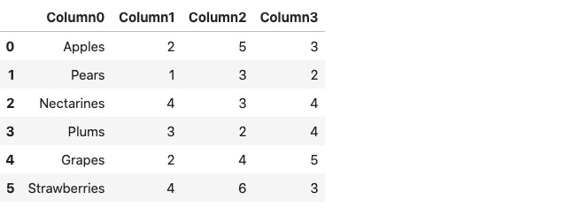
대신에기둥선택한 이름을 지정할 수 있습니다.
3. mangle_dupe_cols
데이터 프레임이 중복 된 열 이름으로 구성된 경우, ‘x’, ‘x’등mangle_dupe_cols.이름을 ‘x’, ‘x1’로 자동 변경하고 반복되는 열을 구별합니다.
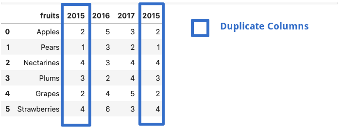
df = pd.read_csv ( 'file.csv', mangle_dupe_cols = true)
Df.
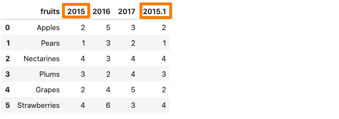
그 중 하나2015 년데이터 프레임의 열은 AS 로의 이름을 삭제합니다2015.1.…에
4. chunksize.
그만큼pandas.read_csv ()기능은 A.chunksize.매개 변수그것은 청크의 크기를 제어합니다.팬더에서 메모리 데이터 집합을로드하는 데 도움이됩니다.chunking을 사용하려면 처음에 청크의 크기를 선언해야합니다.이것은 우리가 반복 할 수있는 객체를 반환합니다.
chunk_size = 5000.
batch_no = 1.
pd.read_csv ( 'yellow_tripdata_2016-02.csv', chunksize = chunk_size)의 chunk의 경우 :
chunk.to_csv ( 'chunk'+ str (batch_no) + '. csv', index = false)
batch_no + = 1.
위의 예에서는 5000의 청크 크기를 선택합니다. 이는 한 번에 5000 줄의 데이터 만 가져올 수 있습니다.우리는 각각 5000 열의 다중 청크를 얻고 각 청크는 팬더 데이터 프레임으로 쉽게로드 될 수 있습니다.
df1 = pd.read_csv ( 'chunk1.csv')
df1.head ()
아래에 설명 된 기사에서 청킹에 대해 자세히 알아볼 수 있습니다.
5. 압축
많은 시간, 우리는 압축 된 파일을받습니다.잘,pandas.read_csv.이러한 압축 파일을 쉽게 처리 할 필요없이 쉽게 처리 할 수 있습니다.기본적으로 압축 매개 변수는 다음으로 설정됩니다미루다,자동으로 파일의 종류를 추론 할 수 있습니다그물,지퍼,BZ2.,xz.파일 확장명에서.
df = pd.read_csv ( 'sample.zip')또는 긴 형태 :df = pd.read_csv ( 'sample.zip', 압축 = 'zip')
6. thousands
데이터 집합의 열에 A.천분리 기호,pandas.read_csv ()그것을 정수가 아닌 문자열로 읽습니다.예를 들어 판매 열에 쉼표 구분 기호가 포함 된 위치에있는 데이터 집합을 고려하십시오.
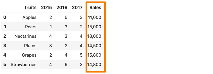
이제 위의 데이터 집합을 팬더 데이터 프레임으로 읽으려면매상열은 쉼표로 인해 문자열로 간주됩니다.
df = pd.read_csv ( 'sample.csv')
df.dtypes.
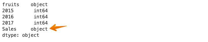
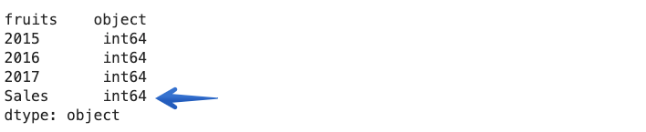
이것을 피하기 위해, 우리는 명시 적으로pandas.read_csv ()쉼표는 쉼표가 수천 개의 장소 표시기입니다.수천 명의매개 변수.
df = pd.read_csv ( 'sample.csv', 수천 = ',')
df.dtypes.
7. skip_blank_lines
빈 줄이 데이터 집합에 있으면 자동으로 건너 뜁니다.빈 줄을 NAN으로 해석하도록 원한다면skip_blank_lines.옵션은 false입니다.
8. 여러 CSV 파일을 읽습니다
이것은 매개 변수가 아니지만 유용한 팁입니다.팬더를 사용하여 여러 파일을 읽으려면 일반적으로 별도의 데이터 프레임이 필요합니다.예를 들어 아래 예제에서는 우리는pd.read_csv ()두 개의 별도의 파일을 두 개의 별개의 데이터 프레임으로 읽으려면 두 번 기능을 수행하십시오.
DF1 = PD.READ_CSV ( 'DATASET1.CSV')
df2 = pd.read_csv ( 'dataset2.csv')
이러한 여러 파일을 함께 읽는 한 가지 방법은 루프를 사용하는 것입니다.다음과 같이 파일 경로 목록을 만들고 목록을 반복합니다.
filenames = [ 'dataset1.csv', 'dataset2, csv']
데이터 프레임 = FILENAMES의 f에 대한 [PD.READ_CSV (f)]
많은 파일 이름이 비슷한 패턴을 가지고있을 때지구본파이썬 표준 라이브러리의 모듈은 편리합니다.우리는 먼저 그를 수입해야합니다지구본내장에서 기능지구본기준 치수.우리는 패턴을 사용합니다멋진 * .csv.접두사로 시작하는 모든 문자열을 일치시킵니다맵시 있는접미사로 끝납니다.csv.그 ‘*'(별표)야생 카드 문자입니다.그것은 0을 포함하여 모든 수의 표준 문자를 나타냅니다.
글로벌 가져 오기
filenames = glob.glob ( '멋진 * .csv')
파일 이름
----------------------------------------------------------------)------------------------------------
[ '멋진 Pharma.csv',
'멋진 it.csv',
'멋진 뱅크 .csv',
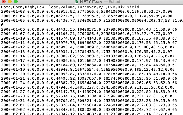
'nifty_data_2020.csv',
'nifty fmcg.csv']
위의 코드를 사용하면 멋진 CSV 파일 이름을 선택할 수 있습니다.이제 목록 이해 또는 루프를 사용하여 모든 것이 즉시 읽을 수 있습니다.
데이터 프레임 = FILENAMES의 f에 대한 [PD.READ_CSV (f)]
Conclusion
이 기사에서는 pandas.read_csv () 함수의 몇 가지 매개 변수를 살펴 보았습니다.그것은 유익한 기능이며 우리가 드물게 사용할 수있는 많은 인구 빌드 매개 변수가 제공됩니다.그렇게하지 않는 주요 이유 중 하나는 문서를 읽을 수 없기 때문입니다.중요한 정보가 포함될 수있는 중요한 정보를 발굴하기 위해 문서를 자세히 설명하는 것이 좋습니다.
There is more to ‘pandas.read_csv()’ than meets the eye
Tips and Tricks
There is more to ‘pandas.read_csv()’ than meets the eye
A deep dive into some of the parameters of the read_csv function in pandas
Pandas is one of the most widely used libraries in the Data Science ecosystem. This versatile library gives us tools to read, explore and manipulate data in Python. The primary tool used for data import in pandas is read_csv().This function accepts the file path of a comma-separated value, a.k.a, CSV file as input, and directly returns a panda’s dataframe. A comma-separated values (CSV) file is a delimited text file that uses a comma to separate values.
The pandas.read_csv()has about 50 optional calling parameters permitting very fine-tuned data import. This article will touch upon some of the lesser-known parameters and their usage in data analysis tasks.
pandas.read_csv() parameters
The syntax for importing a CSV file in pandas using default parameters is as follows:
import pandas as pd
df = pd.read_csv(filepath)
1. verbose
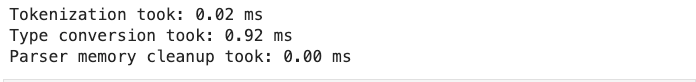
The verbose parameter, when set to True prints additional information on reading a CSV file like time taken for:
- type conversion,
- memory cleanup, and
- tokenization.
import pandas as pd
df = pd.read_csv('fruits.csv',verbose=True)
2. Prefix
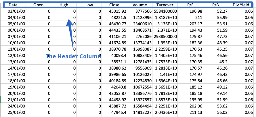
The header is a row in a CSV file containing information about the contents in every column. As the name suggests, it appears at the top of the file.
Sometimes a dataset doesn’t contain a header. To read such files, we have to set the header parameter to none explicitly; else, the first row will be considered the header.
df = pd.read_csv('fruits.csv',header=none)
df
The resulting dataframe consists of column numbers in place of column names, starting from zero. Alternatively, we can use the prefix parameter to generate a prefix to be added to the column numbers.
df = pd.read_csv('fruits.csv',header=None, prefix = 'Column')
df
Note that instead of Column, you can specify any name of your choice.
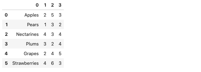
3. mangle_dupe_cols
If a dataframe consists of duplicate column names — ‘X’,’ X’ etcmangle_dupe_cols automatically changes the name to ‘X’, ‘X1’ and differentiate between the repeated columns.
df = pd.read_csv('file.csv',mangle_dupe_cols=True)
df
One of the 2015 column in the dataframe get renames as 2015.1.
4. chunksize
The pandas.read_csv() function comes with a chunksize parameter that controls the size of the chunk. It is helpful in loading out of memory datasets in pandas. To enable chunking, we need to declare the size of the chunk in the beginning. This returns an object we can iterate over.
chunk_size=5000
batch_no=1
for chunk in pd.read_csv('yellow_tripdata_2016-02.csv',chunksize=chunk_size):
    chunk.to_csv('chunk'+str(batch_no)+'.csv',index=False)
    batch_no+=1
In the example above, we choose a chunk size of 5000, which means at a time, only 5000 rows of data will be imported. We obtain multiple chunks of 5000 rows of data each, and each chunk can easily be loaded as a pandas dataframe.
df1 = pd.read_csv('chunk1.csv')
df1.head()
You can read more about chunking in the article mentioned below:
5. compression
A lot of times, we receive compressed files. Well, pandas.read_csv can handle these compressed files easily without the need to uncompress them. The compression parameter by default is set to infer, which can automatically infer the kind of files i.e gzip , zip , bz2 , xz from the file extension.
df = pd.read_csv('sample.zip') or the long form:df = pd.read_csv('sample.zip', compression='zip')
6. thousands
Whenever a column in the dataset contains a thousand separator, pandas.read_csv() reads it as a string rather than an integer. For instance, consider the dataset below where the sales column contains a comma separator.
Now, if we were to read the above dataset into a pandas dataframe, the Sales column would be considered as a string due to the comma.
df = pd.read_csv('sample.csv')
df.dtypes
To avoid this, we need to explicitly tell the pandas.read_csv() function that comma is a thousand place indicator with the help of the thousands parameter.
df = pd.read_csv('sample.csv',thousands=',')
df.dtypes
7. skip_blank_lines
If blank lines are present in a dataset, they are automatically skipped. If you want the blank lines to be interpreted as NaN, set the skip_blank_lines option to False.
8. Reading multiple CSV files
This is not a parameter but just a helpful tip. To read multiple files using pandas, we generally need separate data frames. For example, in the example below, we call the pd.read_csv() function twice to read two separate files into two distinct data frames.
df1 = pd.read_csv('dataset1.csv')
df2 = pd.read_csv('dataset2.csv')
One way of reading these multiple files together would be by using a loop. We’ll create a list of the file paths and then iterate through the list using a list comprehension, as follows:
filenames = ['dataset1.csv', 'dataset2,csv']
dataframes = [pd.read_csv(f) for f in filenames]
When many file names have a similar pattern, the glob module from the Python standard library comes in handy. We first need to import the glob function from the built-in glob module. We use the pattern NIFTY*.csv to match any strings that start with the prefix NIFTY and end with the suffix .CSV. The ‘*’(asterisk) is a wild card character. It represents any number of standard characters, including zero.
import glob
filenames = glob.glob('NIFTY*.csv')
filenames
--------------------------------------------------------------------
['NIFTY PHARMA.csv',
 'NIFTY IT.csv',
 'NIFTY BANK.csv',
 'NIFTY_data_2020.csv',
 'NIFTY FMCG.csv']
The code above makes it possible to select all CSV filenames beginning with NIFTY. Now, they all can be read at once using the list comprehension or a loop.
dataframes = [pd.read_csv(f) for f in filenames]
Conclusion
In this article, we looked at a few parameters of the pandas.read_csv() function. it is a beneficial function and comes with a lot of inbuilt parameters which we seldom use. One of the primary reasons for not doing so is because we rarely care to read the documentation. It is a great idea to explore the documentation in detail to unearth the vital information that it may contain.