불균형 주문서가 책의 얇은면으로 가격 변동을 유발하는지 조사합니다.즉,이 가설에 의해 지정가 주문 장부가 입찰 측에 비해 호가 측에 게시 된 양이 많을 때 가격이 하락하고, 주문 장부가 입찰 측에서 더 무거 우면 가격이 상승합니다.우리는이 가설을 테스트하고 주문 장 불균형 정보를 이용하여 ETHUSD 시장의 가격 변동을 수익성있게 예측할 수 있는지 평가합니다.
주문 장 불균형
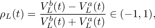
우리는 문헌을 따릅니다.Cartea et al.(2015), 주문 장 불균형을 다음과 같이 정의하십시오.
방정식 1
어디티시간을 인덱싱하고,V입찰 (위 첨자비) 또는 질문 (위첨자ㅏ) 및엘ρ를 계산하기 위해 고려되는 주문서의 깊이 수준입니다..그림 1은 불균형을 계산하는 방법의 예를 보여줍니다.ρ주어진 주문서에 대해.
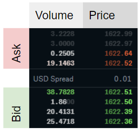
그림 1 : 주문 장 불균형.L = 4의 깊이를 보여주는 Coinbase 웹 사이트의 스크린 샷을 기반으로 한 ETHUSD에 대한 지정가 주문서의 예.L = 1의 불균형은 (38.7828–19.1463) / (38.7828 + 19.1463) ≈ 0.33으로 계산됩니다.이 기사에서 조사한 가설에 따르면 0보다 큰 값은 가격 상승 압력에 해당합니다.L = 2의 경우 불균형을 계산하기 위해 2 개의 최적 가격, 즉 (38.7828 + 1.86–19.1463-0.2505) / (38.7828 + 1.86 + 19.1463 + 0.2505) ≈ 0.36을 더합니다.
ㅏρ-1에 가까운-값은 시장 조성자가 입찰 수량에 비해 대량의 수량을 게시 할 때 획득됩니다.ρ 값이 1에 가까우면 요청 측에 비해 주문서의 입찰 측에 대량이 있음을 의미합니다.불균형이 0이면 주문서가 주어진 수준에서 완벽하게 균형을 이룹니다.엘.가설은 낮은 불균형 숫자 (& lt; 0)는 음의 수익을 의미하고, 높은 불균형 숫자 (& gt; 0)는 양의 수익을 의미합니다. 즉, 가격이 불균형 방향으로 이동 함ρ.
연구자들은 주식 시장 데이터에서 무엇을 결론 내립니까?
Cont et al.(2014)미국 주식 데이터를 사용하여 주문 흐름 불균형의 가격 영향과 “주문 흐름 불균형”과 가격 변동 사이의 선형 관계가 있음을 보여줍니다.저자는 주문 흐름 불균형을 주어진 기간 동안 들어오는 주문을 집계하여 측정 된 공급과 수요 사이의 불균형으로 정의합니다.선형 모델의 R²는 약 70 %입니다.이 연구는 과거 주문 흐름 (불균형 측정을 초래 함)을 고려하고이를 동일한 기간 동안의 가격 변동과 비교합니다.따라서 결론은 주문 흐름 불균형이 미래 가격을 예측하는 것이 아니라 과거 기간 동안 계산 된 주문 흐름 불균형이 같은 기간 동안의 가격 변화를 설명한다는 것입니다.따라서이 연구는 미래 가격에 대한 현재 주문 흐름 불균형에 대한 직접적인 통찰력을 보여주지 않습니다.실란 티 예프 (2018)미디엄 기사에서 BTC-USD 주문서 데이터를 사용하여이 연구 결과를 확인합니다.
Lipton et al.(2013), 우리 불균형 측정ρ와L = 1다음 틱까지의 가격 변동은 주문 장 불균형의 선형 함수에 의해 잘 근사화 될 수 있지만 (1) 변경이 매도 매도 스프레드보다 훨씬 낮고 (2) 방법은 “그 자체로는 직접적인 통계적 차익 거래 기회를 제공하지 않습니다”.
Cartea et al.(2018)에 의해 측정 된 더 높은 주문 책 불균형을 발견하십시오ρ그 뒤에는 시장 주문량이 증가하고 불균형은 시장 주문이 도착한 직후 가격 변화를 예측하는 데 도움이됩니다.
그들의 책에서Cartea et al.(2015)과거 불균형과 가격 변동의 상관 관계가 괜찮은 특정 주식에 대해 존재합니다 (10 초 간격 동안 약 25 %).
스토이 코프 (2017)통합하는 중간 가격 조정을 정의합니다. 주문 장 불균형 및 매도 매도 스프레드.그는 결과가 가격 (중가 + 조정)은 중가 및 볼륨 가중 중가보다 중가의 단기 변동에 대한 더 나은 예측 변수입니다.이 연구에서 주문 장 불균형은 우리의 불균형과 약간 다릅니다. 특히 공식 (1)은 지명자에서 요청 볼륨을 제거하고 레벨을 고정하여 조정됩니다.엘이 방법은 현재 정보를 조건으로 미래의 중간 가격에 대한 기대치를 추정하며 수평선과 무관합니다.예측이 가장 정확한 경험적 지평은 평가 된 주식에 대해 3 ~ 10 초 범위입니다.조정 된 중간 가격은 제시된 데이터에 대한 입찰과 요청 사이에 존재하며, 이는 방법 자체가 통계적 차익 거래 방법을 제시하지 않지만 저자가 언급했듯이 알고리즘을 개선하는 데 사용할 수 있음을 나타냅니다.
이 연구에서는 최적의 매도 호가 가격 (L = 1), 우리는 더 긴 수평선을보고 순서를 계산하기 위해 깊이 5를 조사합니다. 불균형.이 연구의 데이터는 주식 시장 데이터를 사용합니다. 주목할만한 예외실란 티 예프 (2018), 우리는 암호 화폐 주문서를 조사합니다.
데이터
오더 북 데이터는 암호 화폐 거래소에서 공개 API를 통해 조회 할 수 있습니다.캔들 데이터 이외의 과거 데이터는 일반적으로 사용할 수 없습니다.따라서 2019 년 5 월부터 12 월까지 (2019–05–21 01:46:37 ~ 2019–12–18 18:40:59) 10 초 간격으로 Coinbase에서 ETHUSD에 대한 주문 장 데이터를 최대 5 단계까지 수집했습니다.이것은 1,920,617 개의 관측치에 해당합니다.데이터에 약간의 차이가 있습니다 (예 : 시스템 다운 타임으로 인해 분석에서 설명 함).두 개의 후속 주문서 관찰 간의 타임 스탬프 차이가 11 초보다 큰 592 개의 간격을 계산합니다.두 주문서 사이의 타임 스탬프는 연속적인 Websocket 스트림이 아닌 반복적 인 REST 요청을 사용하여 데이터를 수집했기 때문에 데이터에서 정확히 10 초가 아닙니다.
오더 북 불균형 분배
가격 변동과 주문 장 불균형 간의 관계를 살펴보기 전에 다양한 주문 장 수준에 대한 불균형 분포를 살펴 봅니다.
주문 장 불균형을 계산합니다.ρ모든 관측치와 방정식 1에 따라 5 가지 레벨에 대해 다음 속성을 찾습니다.
에서L = 1불균형은 종종 매우 뚜렷하거나 전혀 존재하지 않습니다.더 높이엘, 균형 잡힌 주문 장부가 더 빈번할수록 (즉,ρ≈0).
불균형은 자기 상관입니다.레벨이 깊을수록엘, 자기 상관이 높을수록
그림 2와 3에서 첫 번째 결과를, 그림 4에서 두 번째 결과를 제시합니다.
그림 2는 레벨 1에 대한 오더 북 불균형의 히스토그램을 보여줍니다.이 레벨에서 오더 북은 대부분 균형이 잡혀 있거나 (0에 가까움) 매우 불균형 (-1 또는 1에 가까움)되어 있습니다.
그림 2 : 주문 장 불균형의 히스토그램.이 그림은 레벨 1의 불균형을 보여줍니다. 즉, 불균형을 계산하기 위해 최적가와 최적가 만 고려한 것입니다.
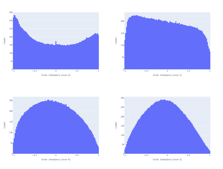
불균형을 계산하기 위해 주문 장 깊이를 늘리면 그림 3에서 볼 수 있듯이 주문 장의 균형이 더 높아집니다.
그림 3 : 다양한 주문 장 깊이에 대한 주문 장 불균형.이 그림은 레벨 2 (왼쪽 상단), 3 (오른쪽 상단), 4 (왼쪽 하단) 및 5의 불균형을 보여줍니다. 더 많은 수준의 깊이를 고려할 때 주문서가 더 균형을 이룹니다.
그림 4는 자기 상관 함수 (ACF)를 보여줍니다.일치Cuartea et al.(2015)불균형은 자기 상관성이 높다는 것을 알 수 있습니다.주어진 지연에 대한 상관 관계는 더 높은 경향이 있으며 주문 장 깊이가 더 큽니다.엘불균형 계산을 위해.
그림 4 : 고정 주문 장 불균형.상단 플롯은 레벨 1에서 계산 된 불균형에 대한 자기 상관 함수를 보여줍니다. 하단은 레벨 5에 대해 계산 된 불균형에 대한 자기 상관 함수를 보여줍니다. 불균형을 계산할 때 깊이를 늘리면 주문 장 불균형의 자기 상관이 더 높습니다.
주문 장 불균형이 가격 변동을 예측하는 데 도움이됩니까?
이제 ρ와 미래 중간 가격의 상관 관계를 조사합니다.중간 가격은 최고 입찰 가격과 최저 요청 가격의 평균으로 정의됩니다.
먼저 주문 장 불균형을 관찰 할 때마다 중간 가격의 p- 기간 선행 로그 수익을 계산합니다.그런 다음 이러한 수익률과 기간 초에 관찰 된 주문 불균형 간의 상관 관계를 계산합니다.p-주기가 평균 11 초 (1주기 ≈ 10 초)보다 긴 관측치를 제거합니다.
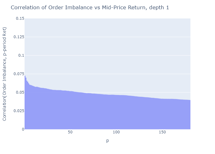
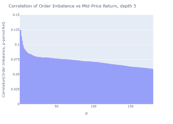
그림 5와 6은 수익이 측정되는 기간의 함수로서 미래 수익률과 불균형의 상관 관계를 보여줍니다.우리는 다음과 같이 결론을 내립니다.
상관 관계가 낮습니다. 예 :Cont et al.(2014)가격 영향과 동일한 기간 동안의 주문 흐름 불균형 측정 사이에 약 70 %의 R²를보고합니다.선형 일 변량 회귀 모델의 경우R²는 상관 관계를 의미합니다.sqrt의(0.70) = 0.84.그러나 저자는 가격 인상을같은 기간주문 흐름 불균형으로 인해이 방법은 가격 예측을 제공하지 않습니다.
불균형 측정ρ불균형 관찰에 가까운 가격에 대해 더 예측 가능합니다 (p가 증가하면 상관 관계가 감소 함).
깊이 수준이 높을수록엘불균형을 계산하기 위해 고려되는 주문서의 불균형 측정치가 미래 가격 변동과 더 많이 연관 됨
그림 5 : 주문 불균형 (L = 1)과 중간 가격 수익률을 앞선 p 기간의 상관 관계.불균형 측정 값과 수익률의 상관 관계는 단기 가격에서 가장 높습니다.
그림 6 : 주문 불균형 (L = 5)과 중간 가격 수익률을 앞선 p 기간의 상관 관계.그림 5와 비교할 때 데이터는 더 깊은 주문 장 레벨 (L)로 계산 된 주문 장 불균형이 낮은 L로 계산 된 것보다 더 나은 가격 예측 변수임을 시사합니다.
깊이에 대한 해당 플롯L = 2…에4간결하게 보여주지 않는 것은 이러한 결과와 일치합니다.이러한 플롯에 대한 Python 코드는 부록 A2를 참조하십시오.
가격 불확실성
위에 제시된 상관 관계는 불균형이 더 높은엘낮은 가격으로 계산 된 불균형보다 가격 상승과 더 나은 상관 관계엘.더 많은 단기 가격은 ρ와 더 높은 상관 관계를 갖습니다.이를 바탕으로 우리는 한 기간 앞선 예측 (≈10 초)만으로 분석을 계속합니다.
상관 관계는 평균 측정 값입니다. 중간 가격 움직임의 불확실성은 어떻습니까?
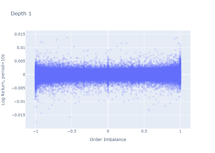
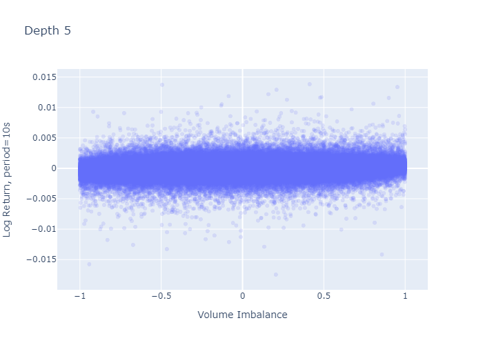
그림 7과 8은 기간 초에 관찰 된 불균형에 대한 1주기 로그 수익률을 보여줍니다.L = 1과L = 5각기.레벨 1 불균형 플롯 (그림 7)은 불균형이 크거나 (-1에 가까움 또는 1에 가까움) 0 일 때 로그 반환의 더 큰 변동이있는 것처럼 보이며, 이는 레벨 5 불균형에 대해 관찰되지 않습니다 (그림 8).그러나이 플롯의 더 큰 변동은 경계와 0 (그림 2 및 3의 히스토그램에서 볼 수 있음)에서 L = 1에 대해 더 많은 관측치를 가지고 있다는 사실에서 기인합니다. 수익률의 표준 편차를 계산해도 더 높은 것이 확인되지는 않습니다.다음 단락에서 볼 수 있듯이 극단에서의 차이.
그림 7 : L = 1에 대한 1주기 수익률 대 불균형.플롯의 각 점은 주문 불균형 (x 축)을 관찰 한 후 한 기간 동안 관찰 된 수익률 (y 축)을 나타냅니다.
그림 8 : L = 5에 대한 한 기간 수익률 대 불균형.
불균형 체제
우리는 따른다Cartea et al.(2018)불균형 측정 값을 지점을 따라 균등하게 배치되도록 선택한 5 개 체제로 분류합니다.
θ = {-1, -0.6, -0.2, 0.2, 0.6, 1}.
즉, 정권 0은 -1과 -0.6 사이의 가격 불균형을 가지고 있고, 정권 1은 -0.6에서 -0.2까지 등등입니다.표 1은 5 개 체제 모두에 대한 1주기 선행 가격 수익률의 표준 편차를 보여줍니다.
표 1 : 정권 당 1 기 중간 가격 수익률의 표준 편차.
표 1은 이전 단락의 질문을 다룹니다. 극심한 불균형 (정권 0 및 정권 4)에서 중간 가격 차이는 다음과 같습니다.아니주문 장 깊이 레벨 L = 1이 레벨 5보다 높습니다.
이제 우리는이 분석을 추가로 취하고 신뢰 구간을 구성하여 주어진 체제에서 예상되는 중간 가격 수익률에 대한 확률 적 한계를 추정합니다.이 계산에 대한 자세한 내용은 부록 A1에 나와 있습니다.
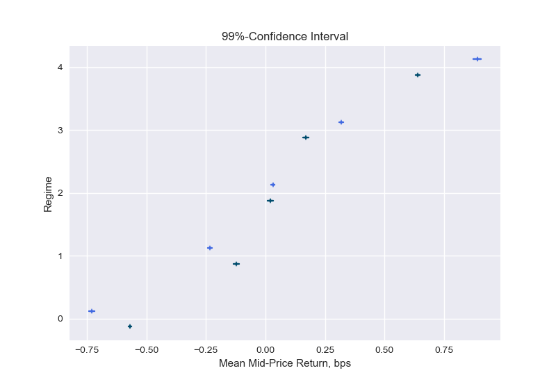
그림 9 : 레벨 1 (어두움) 및 5 (밝음) 불균형에 대한 예상 중간 가격 수익률에 대한 신뢰 구간.수직 마커는 기대 수익의 포인트 추정치를 보여주고, 수평선은 기대 수익의 99 % 신뢰 구간의 경계를 나타냅니다.진한 선은 불균형 수준 1의 간격을, 밝은 선은 수준 5의 간격을 나타냅니다.
그림 9는 주어진 체제에서 예상되는 중간 가격 수익률에 대한 신뢰 구간을 보여줍니다.실제로 수익률은 낮은 불균형 수 (정권 0 및 1)에 대해 평균 음수이고 높은 불균형 수 (정규 3 및 4)에 대해 양수임을 알 수 있습니다.불균형이 더 높은 수준으로 구성 될 때 평균은 순서 불균형 방향으로 더 많이 이동합니다. 예를 들어, 영역 4에서 불균형이 다음과 같이 계산 될 때 1주기 선행 수익의 평균L = 1(진한 선)은 레벨의 깊이에서 계산을 수행 할 때보 다 작습니다.L = 5(밝은 선).표시된 신뢰 구간은 예상 값의 불확실성을 반영합니다.표 1의 표준 편차는이 예상 값 주변 수익률의 불확실성에 대해 알려줍니다.
이 분석은 상관 분석의 결과를 확인합니다. 불균형과 1주기 선행 수익 사이에는 양의 상관 관계가 있지만 약한 상관 관계가 있으며, 더 깊은 수준 (L)은 약간 더 예측 가능한 불균형 측정을 생성합니다.
경험적 확률
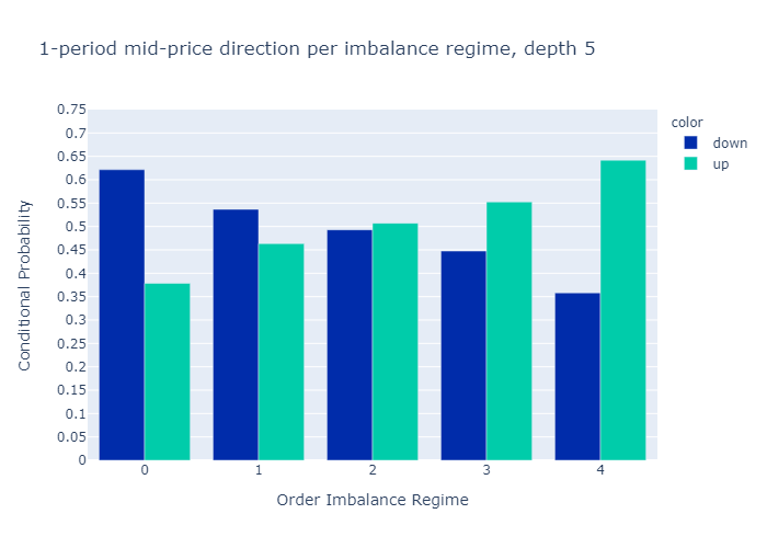
다음 기간 중간 가격이 우리가 어떤 불균형 체제에 속해 있는지 알면서 상승, 고정 또는 하락할 확률은 얼마입니까?
이를 확인하기 위해 모든 주문 불균형을 영역 0-4로 버킷 화 한 다음 음수 수익률, 0 수익률 및 양의 1 기간 수익률을 계산하고이 개수를 관측치 수로 나누어 확률에 대한 추정치를 구합니다.중간 가격 움직임.
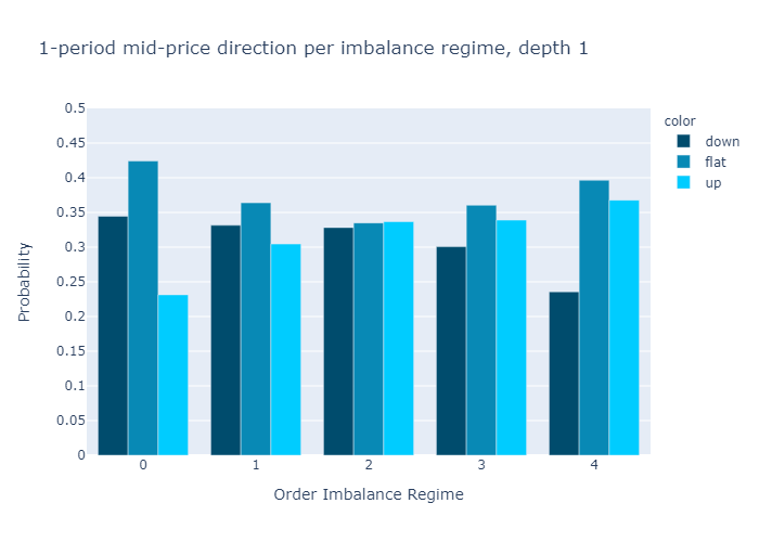
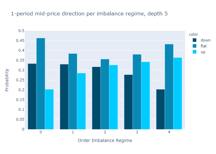
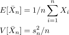
그림 10과 11은 다음에 대해 계산 된 불균형에 대한 경험적 확률을 보여줍니다.L = 1과L = 5각기.수치는 우리의 초기 가설을 확인합니다.
주문 장 불균형 값이 낮은 제도에서는 중간 가격이 하락할 가능성이 더 높으며 그 반대의 경우도 마찬가지입니다.
1 단계 (그림 10) 또는 5 단계 (그림 11)만으로 불균형을 계산할 때 경험적 확률에 질적으로 차이가 없음을 알 수 있습니다.우리는 더 높은 수준에 대한 확률이L = 5보다 차별적이다L = 1, 이는 원하는 속성입니다.
부록 A3에서 우리는 또한 0이 아닌 가격 변동을 관찰 할 때 조건부 확률을 보여줍니다.가격이 움직이면 레벨 5 불균형이 레벨 1 불균형보다 약간 더 나은 예측 변수입니다.
많은 암호 화폐 거래소에는 10bps의 거래 수수료가 있습니다 (그리고 우리는 2 번의 거래를 실행할 것입니다).신뢰 구간 (그림 9)에서 고려한 10 초 기간 동안 중간 가격 수익률이 10 베이시스 포인트 미만임을 알 수 있습니다.따라서 차이를 고려하지 않고 기대 수익률로 판단하면 주문 불균형이 매도-매도 스프레드를 조사하지 않고서도 자체적으로 수익성있는 전략을 의미하는 것은 아니라는 결론을 내릴 수 있습니다.
이 결과를 확인하기 위해 다른 각도에서 수익성을 살펴보고 그림 10 및 11과 유사하게 10 베이시스 포인트보다 큰 가격 변동의 경험적 확률을 계산합니다. 즉, 절대적으로 10 베이시스 포인트 미만인 모든 움직임을 다음과 같이 계산합니다.플랫.표 3은 주문 장 수준이 1과 5 모두 인 불균형 계산의 경우 대부분의 거래가 모든 체제에서 10 베이시스 포인트의 절대 수익 이하로 끝날 것임을 보여줍니다.이것은 전략이 자체적으로 통계적 차익 거래를 허용하지 않음을 확인합니다.
표 3 : 주문 장 불균형 체제 당 경험적 확률.이 표는 주문 장 불균형 관찰 (정권 0 ~ 4) 후 한 기간 내에 상승, 하락 또는 10bps (플랫)보다 작은 상대 이동에 대한 경험적 확률을 보여줍니다.열 확률 L1은 레벨 1 주문 장 불균형에 대해 계산 된 경험적 확률과 레벨 5 주문 장 불균형에 대해 L5를 보여줍니다.
결론
ETHUSD 주문 장 및 중간 가격 움직임에 대한 우리의 분석은 주식 시장의 주문 장 불균형에 대한 문헌의 결과와 일치합니다.
불균형이 -1에 가까울 때 매도 압력이 있고 단기적으로 중가가 하락할 가능성이 더 높고, 불균형이 1에 가까울 때 매수 압력이 있고 중간 가격이이동.
불균형 조치의 가격 영향은 수명이 짧으며 시간이 지남에 따라 빠르게 악화됩니다.
불균형 측정 자체는 통계적 차익 거래에 직접 사용할 수 없지만 알고리즘을 개선하는 데 사용할 수 있습니다.
오더 북 불균형에 대한 문헌에서 인용 한 것 외에도 최대 5 개 레벨을 사용하여 계산 된 오더 북 불균형을 분석 한 결과 불균형 측정 값과 미래 가격 움직임과의 상관 관계가 레벨에 따라 증가한다는 것을 발견했습니다 (평가 된 5 개 레벨에 대해)..그러나 그림 9의 기대 값과 신뢰 구간에서 높은 수준은 수익 방향을 약간 개선 할 뿐이며, 더 높은 수준의 주문 장 깊이로 작업 할 때 경험적 확률이 약간 더 차별적이라는 것을 관찰했습니다.따라서, 더 깊은 레벨 (L & gt; 1)에서 추가 된 값은 아마도 더 높은 복잡성을 정당화하지 않을 것입니다 (더 깊은 레벨을 처리하는 것은 일반적으로 고주파 알고리즘에 대해 더 많은 시간이 소요됨).
마지막으로 불균형과 가격 변동 사이의 가장 강력한 관계가 데이터에서 사용할 수있는 가장 짧은 기간 (10 초) 내에 있음을 발견했습니다.따라서 틱 데이터를 살펴보면이 기사에서 살펴본 10 초의 기간과 달리 더 많은 통찰력을 얻을 수 있다고 결론지었습니다.
참고 문헌
Cartea, A., R. Donnelly 및 S. Jaimungal (2018).주문 장 신호로 거래 전략을 강화합니다.응용 수학 금융25 (1), 1-35.
Cartea, A., S. Jaimungal 및 J. Penalva (2015).알고리즘 및 고주파 거래.캠브리지 대학 출판부.
Cont, R., A. Kukanov 및 S. Stoikov (2014).오더 북 이벤트의 가격 영향.Journal of Financial Econometrics12 (1), 47-88.
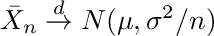
어디Xi대표하다i = 1,…, n평균이있는 분포에서 도출 된 관측치μ및 표준 편차σ, 위첨자가있는 화살표디분포 수렴을 나타내고 N (0,1)은 표준 정규 분포를 나타냅니다.방정식 A.2를 표현할 수 있습니다.비공식적으로
방정식 A.3
평균과 분산의 추정치로 이어지는
방정식 A.4
어디에스표본 표준 편차입니다.이제 수준 (1-α)에 대한 신뢰 구간은 다음과 같이 지정됩니다.
방정식 A.5
z (α)다음보다 큰 값을 관찰 할 확률이되도록 표준 정규 밀도 곡선의 x 축에있는 점을 나타냅니다.z (α)이하-z (α)α와 같습니다.
이 형태의 중앙 한계 정리를 적용하려면 중간 가격 수익률이i.i.d..중간 가격 수익률의 자기 상관은 1 % 미만이며 (A2 참조) 다른 분포에서 비롯되거나 상관 관계에 반영되지 않은 다른 종속성을 가져야한다는 표시가 없으므로 다음을 가정 할 수 있습니다.i.i.d.재산 보유 및 사용 방정식 A.4.
scipy.stats를 st로 가져 오기
numpy를 np로 가져 오기def Estimated_confidence (shifted_return,
vol_binned,
volume_regime_num,
alpha = 0.1) :
    "" "
주어진 알파에 대한 신뢰 구간 추정
    : paramshifted_return : 계산할 반환 배열
신뢰 구간
평균의 NaN 포함 가능
    :유형shifted_return : 길이 n의 부동 소수점 배열
    : paramvol_binned : 볼륨 체제.항목 i는
                       volume regime associated with
                       shifted_return[i]
    :typevol_binned : 길이 n의 부동 배열
    : param volume_regime_num: equals np.max(vol_binned)+1
    :유형volume_regime_num : 정수
    :반환: confidence intervals for mean of the returns per regime
    : rtype:  float array of size volume_regime_num x 2
    """
    Confident_interval = np.zeros ((volume_regime_num, 2))
z = st.norm.ppf (1- 알파)
    for regime_num in range(0, volume_regime_num):
m = np.nanmean (shifted_return [vol_binned == regime_num])
s = np.nanstd (shifted_return [vol_binned == regime_num])
        sqrt_n = np.sqrt(np.sum(vol_binned == regime_num))
        confidence_interval[regime_num, :] = [m - z * s/sqrt_n,
m + z * s / sqrt_n]
    return confidence_interval
A2. Plot the autocorrelation function
아래의 Python 코드 조각은 자기 상관과 플롯을 계산합니다.계산은 11 초보다 큰 시계열의 (하드 코딩 된) 간격을 설명합니다.
numpy를 np로 가져 오기
datetime 가져 오기 datetime에서
import plotly.express as pxdef shift_array(v, num_shift):
    '' '
배열을 왼쪽 (num_shift & lt; 0) 또는 오른쪽 num_shift & gt; 0으로 이동
    : paramv : 이동할 float 배열
    :유형v : 어레이 1d
    : param num_shift: number of shifts
    :typenum_shift : 정수
    :반환: 원래 배열과 동일한 길이의 부동 배열,
num_shifts 요소로 이동, np.nan
경계의 항목
    : rtype:  array
    '''
    v_shift = np.roll (v, num_shift)
num_shift & gt;0 :
v_shift [: num_shift] = np.nan
그밖에:
v_shift [num_shift :] = np.nan
반환 v_shiftdef plot_acf(v, max_lag, timestamp):
    '' '
자기 상관 함수를 플로팅하기위한 Figure 생성
    :parammax_lag : 자기 상관을 중지 할시기
계산 (최대 max_lag 시차까지)
    : param timestamp: timestamp array of length n
           with entry i corresponding to timestamp of
           entry i in v, used to remove time-jumps
v : n 개의 관측치가있는 배열
    :return: 음모 그림
'' '
    corr_vec = np.zeros (max_lag, dtype = float)
    for k in range(max_lag):
v_lag = shift_array (v, -k-1)
timestamp_lag = shift_array (타임 스탬프, -k-1)
        dT = (timestamp - timestamp_lag) / (k+1)
msk_time_gap = dT & gt;11000.0
마스크 = ~ np.isnan (v) & amp;~ np.isnan (v_lag) & amp;~ msk_time_gap
corr_vec [k] = np.corrcoef (v [마스크], v_lag [마스크]) [0, 1]
fig_acf = px.bar (x = 범위 (1, max_lag + 1), y = corr_vec)
fig_acf.update_layout (yaxis_range = [0, 1])
fig_acf.update_xaxes (title = "Lag")
    fig_acf.update_yaxes(title="ACF")
    return fig_acf
A3. Conditional Empirical Probabilities
그림 A1과 A2는 0이 아닌 수익률을 관찰 할 때 중간 가격 상승 / 하강 이동의 경험적 확률을 보여줍니다.수준 5 불균형은 더 나은 차별 력을 보여줍니다. 즉, 영역 0과 5에서 확률은 수준 1보다 더 극단적입니다.
If the mid-price moves, the imbalance with L=5 is a better indicator of the price direction than the imbalance of L=1.
그림 A1 : 중간 가격 움직임에 대한 조건부 경험적 확률 (불균형 깊이 수준 1).
그림 A2 : 중간 가격 움직임에 대한 조건부 경험적 확률 (불균형 깊이 레벨 5).
Towards Data Science 편집자의 참고 사항 :독립적 인 저자가 우리의규칙 및 지침, 우리는 각 저자의 기여를 보증하지 않습니다.전문적인 조언을 구하지 않고 작가의 작품에 의존해서는 안됩니다.우리를 참조하십시오독자 용어자세한 내용은.
We investigate whether imbalanced order books lead to price changes towards the thinner side of the book. That is, by this hypothesis prices decrease when limit order books have large volumes posted at the ask side relative to the bid side, and if order books are more heavy on the bid side then prices increase. We test this hypothesis and assess whether order book imbalance information can be exploited to profitably predict price movements in the ETHUSD market.
Order book imbalance
We follow the literature, e.g., Cartea et al. (2015), and define the order book imbalance as
Equation 1
where t indexes the time, V stands for volume at either the bid (superscript b) or ask (superscript a), and L is the depth level of the order book considered to calculate ρ. Figure 1 shows an example how to calculate the imbalance ρ for a given order book.
Figure 1: Order Book Imbalance. Example of a limit order book for ETHUSD based on a screenshot from the Coinbase-website showing a depth of L=4. The imbalance for L=1 is calculated as (38.7828–19.1463)/(38.7828+19.1463) ≈ 0.33. By the hypothesis we investigate in this article, a value greater than zero corresponds to a price upward pressure. For L=2 we sum the 2 best prices to calculate the imbalance, that is, (38.7828+1.86–19.1463-0.2505)/(38.7828+1.86+19.1463+0.2505)≈ 0.36.
A ρ-value close to -1 is obtained when market makers post a large volume at the ask relative to the bid volume. A ρ-value close to 1 means there is a large volume at the bid side of the order book relative to the ask side. With an imbalance of zero the order book is perfectly balanced at the given level L. The hypothesis suggests that low imbalance numbers (<0) imply negative returns, high imbalance numbers (>0) imply positive returns, i.e., the price moves into the direction of the imbalance ρ.
What do researchers conclude from stock market data?
Cont et al. (2014) use US stock data to show that there is a price impact of order flow imbalance and a linear relationship between “order flow imbalance” and price changes. The authors define order flow imbalance as the imbalance between supply and demand, measured by aggregating incoming orders over a given period. Their linear model has an R² of around 70%. The study considers the past order flows (that result in an imbalance measure) and compares it to the price change over the same period. Hence, the conclusion is not that order flow imbalances predict future prices, but rather that the order flow imbalances computed over a historic period explains the price change over the same period. So this study reveals no direct insights on current order flow imbalances on future prices. Silantyev (2018) confirms the finding of this study using BTC-USD order book data in his Medium article.
Lipton et al. (2013), us the imbalance measure ρ with L=1 and find that the price change until the next tick can be well approximated by a linear function of the order book imbalance but note that (1) the change is well below the bid-ask spread, and (2) the method “does not by itself offer an opportunity for a straightforward statistical arbitrage”.
Cartea et al. (2018) find that a higher order book imbalance measured by ρ is followed by an increased amount of market orders and that the imbalance helps to predict price changes immediately after the arrival of a market order.
In their book, Cartea et al. (2015) present for one particular stock that correlations of past imbalances and price changes are decent (about 25% for a 10-second interval).
Stoikov (2017) defines a mid-price adjustment that incorporates order book imbalances and bid-ask spreads. He finds that the resulting price (mid-price plus adjustment) is a better predictor for short-term movements of mid-prices than mid-prices and volume-weighted mid-prices. In this study, the order book imbalance slightly differs from ours, specifically Equation (1) would be adjusted by removing the ask volume from the nominator and fixing the level L to 1. The method estimates the expectation of the future mid-price conditional on current information and is horizon independent. Empirically horizons for which the forecasts are most accurate range from 3 to 10 seconds for the stocks assessed. The adjusted mid-price lives between the bid and the ask for the data presented which indicates that the method by itself does not present a method for statistical arbitrage, but as the author notes can be used to improve upon algorithms.
These studies consider tick-level data at the best bid-ask price (L=1), we look at longer horizons and delve into a depth of 5 to calculate the order imbalance. The data in these studies uses stock market data, with the notable exception of Silantyev (2018), whereas we look into cryptocurrency order books.
Data
Order book data can be queried via public API from crypto-exchanges. Historical data other than candle data is not generally available. Hence I collected order book data for ETHUSD from Coinbase in 10 second intervals up to a depth of 5 levels from May to December 2019 (2019–05–21 01:46:37 to 2019–12–18 18:40:59). This amounts to 1,920,617 observations. There are some gaps in the data, e.g., due to system downtimes, which we account for in our analysis. We count 592 gaps where the timestamp difference between two subsequent order book observations is larger than 11 seconds. The timestamp between two order books is not exactly 10 seconds in the data since I collected the data using repeated REST requests, rather than, e.g., a continuous Websocket stream.
Distribution of order book imbalance
Before looking at the relationship between price changes and the order book imbalance, we look at the distribution of the imbalance for different order book levels.
We calculate the order book imbalance ρ for all observations and the 5 different levels according to Equation 1 and find the following properties.
At L=1 the imbalances are often very pronounced or not existent at all. The higher L, the more frequent are balanced order books (i.e., more observations for ρ≈0).
The imbalance is autocorrelated. The deeper the level L, the higher the autocorrelation
We present the first finding in Figures 2 and 3 and the second in Figure 4.
Figure 2 shows a histogram of order book imbalances for level 1. We observe that at this level, the order book is mostly balanced (close to 0), or highly imbalanced (close to -1 or 1).
Figure 2: Histogram of Order Book Imbalances. This figure shows the imbalance at level 1, that is, considering only the best bid and best ask price to calculate the imbalance.
As we increase the order book depth to calculate the imbalance, the order books become more balanced, as we see in Figure 3.
Figure 3: Order Book Imbalances for different order book depths. This figure shows the imbalance at level 2 (top left), 3 (top right), 4(bottom left) and 5. The order book is more balanced when more levels of depth are considered.
Figure 4 shows the autocorrelation function (ACF). Consistent with Cuartea et al. (2015) we find that imbalances are highly autocorrelated. The correlation for a given lag tends to be higher, the larger the order book depth L for the calculation of the imbalance.
Figure 4: Sticky Order Book Imbalances. The top plot shows the autocorrelation function for an imbalance computed at level 1, the bottom the one for level 5. We observe higher autocorrelations of order book imbalances if we increase the depth in calculating the imbalance.
Do order book imbalances help to predict price movements?
We now investigate the correlation of ρ and future mid-prices. Mid-prices are defined as the average of highest bid price and the lowest ask price.
We first calculate the p-period ahead log-return of the mid-price for each observation of order book imbalance. We then calculate the correlation between these returns and the order imbalances observed at the beginning of the period. We remove observations where the p-periods are on average longer than 11 seconds (1 period ≈ 10 seconds).
Figure 5 and 6 show the correlations of future returns and imbalances as a function of the period over which the return is measured. We conclude as follows.
The correlations are low. E.g., Cont et al. (2014) report an R² of about 70% between the price-impact and their measure of order flow imbalance over the same period. For a linear univariate regression model this R² implies a correlation of sqrt(0.70)=0.84. However, the authors measure the price increase over the same period as the order flow imbalance, hence this method does not offer price forecasts
The imbalance measure ρ is more predictive for prices closer to the imbalance observation (the correlation decreases as p increases)
The higher the depth level L of the order book considered to calculate the imbalance, the more the imbalance measure correlates with future price movements
Figure 5: Correlation of p-period ahead mid-price returns with order imbalance (L=1). The correlation of the imbalance measure with return is highest for near-term prices.
Figure 6: Correlation of p-period ahead mid-price returns with order imbalance (L=5). Comparing to Figure 5, the data suggests that order book imbalances computed with a deeper order book level (L) is a better price predictor than the one computed with low L.
The corresponding plots for depths L=2 to 4 which I don’t show for brevity are consistent with these findings. For Python code for these plots see Appendix A2.
Price uncertainty
The correlations presented above showed that imbalances calculated with higher L correlates better with price increases than imbalances calculated with lower L. More near-term prices have a higher correlation with ρ. Based on this we continue the analysis with only one-period ahead forecasts (≈10s).
Correlation is an average measure, what about the uncertainty of the mid-price moves?
Figure 7 and 8 plot the 1-period log-return against the imbalance observed at the beginning of the period for L=1 and L=5 respectively. The level 1 imbalance plot (Figure 7) looks as if there was a higher variation of log-returns when the imbalance is large (close to -1 or close to 1) or 0, which we don’t observe for level 5 imbalances (Figure 8). However, this seemingly larger variation in the plot stems from the fact that we have more observations for L=1 at the boundaries and at zero (seen in the histograms in Figures 2 and 3) — calculating the standard deviation of returns does not confirm higher variances at the extremes as we see in the next paragraph.
Figure 7: One-period Return vs Imbalance for L=1. Each point in the plot represents a return (y-axis) observed over one period after observing the order imbalance (x-axis)
Figure 8: One-period Return vs Imbalance for L=5.
Imbalance regimes
We follow Cartea et al. (2018) and bucket our imbalance measure into five regimes chosen to be equally spaced along the points
θ = {-1, -0.6, -0.2, 0.2, 0.6, 1}.
That is, regime 0 has price imbalances between -1 and -0.6, regime 1 from -0.6 to -0.2 and so on. Table 1 shows the standard deviation of 1-period ahead price returns for all 5 regimes.
Table 1: Standard deviation of 1-period mid-price returns per regime.
Table 1 addresses the question from the previous paragraph: the mid-price variance at extreme imbalances (regime 0 and regime 4) is not higher for order book depth level L=1 than for level 5.
Now we take this analysis further and estimate probabilistic bounds for the expected mid-price return in a given regime by constructing confidence intervals. I provide details on this calculation in Appendix A1.
Figure 9: Confidence intervals for expected mid-price returns for level 1 (dark) and 5 (bright) imbalances. The vertical markers show the point estimate of the expected return, the horizontal lines represent the boundaries of the 99%-confidence interval of the expected return. The dark lines shows the intervals for imbalance level 1, the brighter lines the one for level 5.
Figure 9 presents confidence intervals for the expected mid-price return in a given regime. We can see that indeed the returns are on average negative for low imbalance numbers (regime 0 and 1) and positive for high imbalance numbers (regime 3 and 4). The means move more into the order imbalance direction when the imbalance is constructed with a higher level, e.g., in regime 4 the mean of the 1-period ahead return when the imbalance is calculated with L=1 (dark line) is smaller than when performing the calculations at a depth of level L=5 (bright line). Note that the confidence intervals shown reflect the uncertainty in the expected value. The standard deviations of Table 1 inform us about the uncertainty of the returns around this expected value.
This analysis confirms the findings from the correlation analysis: there is positive but weak correlation between imbalances and 1-period ahead returns, and the deeper level (L) results in a slightly more predictive imbalance measure.
Empirical probabilities
What is the probability that the next period mid-price will go up, stay flat, or go down knowing in which imbalance regime we are?
To see this, we bucket every order imbalance into a regime 0-4 and then count the number of negative returns, zero returns, and positive 1-period returns and divide the count by the number of observation to have an estimate for the probabilities of mid-price moves.
Figures 10 and 11 present the empirical probabilities for imbalances computed for L=1 and L=5 respectively. The figures confirm our initial hypothesis:
There is a higher probability of mid-price decreases in regimes with low values of order book imbalance, and vice versa.
We see qualitatively no difference in the empirical probabilities when calculating the imbalances with only 1 level (Figure 10) or 5 levels (Figure 11). We observe that the probabilities for higher levels L=5 are more discriminatory than for L=1, which is a desired property.
In Appendix A3 we also show the probabilities conditional on observing a non-zero price move. We find that if the price moves, the level 5 imbalance is a slightly better predictor than the level 1 imbalance.
Figure 10: Empirical Probability for Mid-Price Move at L=1.
Figure 11: Empirical Probability for Mid-Price Move at L=5.
Many crypto exchanges have trading fees in the order of 10bps (and we would execute 2 trades). We see from the confidence intervals (Figure 9) that mid-price returns are below 10 basis points for the 10 second periods considered. So from judging by the expected return without considering variances, we can conclude that order imbalances do not directly imply a profitable strategy on its own without even investigating the bid-ask spreads.
To affirm this finding, we look at profitability from another angle and calculate the empirical probabilities of price moves larger than 10 basis points, similar to figures 10 and 11. That is, we count all movements that are in absolute terms below 10 basis points as flat. Table 3 shows that for imbalance calculations with order book levels of both 1 and 5, most trades would end up below an absolute return of 10 basis points in all regimes. This confirms the strategy does not allow for statistical arbitrage on its own.
Table 3: Empirical probabilities per order book imbalance regime. This table shows the empirical probability for up moves, down moves, or relative moves smaller than 10bps (flat) within one period after the order book imbalance observation (regimes 0 to 4). The column probability L1 shows the empirical probabilities computed for Level 1 order book imbalances, and L5 that for level 5 order book imbalances.
Conclusion
Our analysis for ETHUSD order books and mid-price movements is consistent with the findings in the literature on order book imbalances for stock markets:
When the imbalance is close to -1 there is a selling pressure and the mid-price is more likely to go down in the near term, when the imbalance is close to 1 there is a buying pressure and the mid-price is more likely to move up.
The price impact of the imbalance measure is short-lived and quickly deteriorates with the time horizon.
The imbalance measure itself cannot directly be used for statistical arbitrage, however, it can be used to improve upon algorithms.
In addition to what the literature cited on order book imbalances, I have also analyzed the order book imbalance calculated using up to 5 levels and found that the correlation of the imbalance measure with future price moves increases with the level (for the 5 levels assessed). From the expected values and its confidence intervals in Figure 9, however, we see that higher levels do only marginally improve the return direction and we observed that empirical probabilities are only slightly more discriminatory when working with higher levels of order book depths. Therefore, the added value from deeper levels (L>1) does probably not justify the higher complexity (handling deeper levels is typically more time consuming for high frequency algorithms).
Finally, we found the strongest relationship between imbalance and price movements to be within the shortest period (10 seconds) available in the data. Therefore, I conclude that looking into tick data could reveal more insights, as opposed to the 10 second period length examined in this article.
References
Cartea, A., R. Donnelly, and S. Jaimungal (2018). Enhancing trading strategies with order book signals. Applied Mathematical Finance 25 (1), 1-35.
Cartea, A., S. Jaimungal, and J. Penalva (2015). Algorithmic and high-frequency trading. Cambridge University Press.
Cont, R., A. Kukanov, and S. Stoikov (2014). The price impact of order book events. Journal of financial econometrics 12 (1), 47-88.
Lipton, A., U. Pesavento, and M. G. Sotiropoulos (2013). Trade arrival dynamics and quote imbalance in a limit order book. arXiv preprint arXiv:1312.0514 .
Paolella, M. S. (2007). Intermediate probability: A computational approach. John Wiley & Sons.
Stoikov, S. (2017). The micro-price: A high frequency estimator of future prices. Available at SSRN 2970694 .
Appendix
A1. Confidence intervals
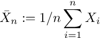
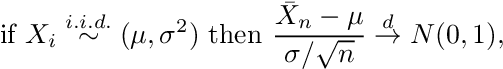
We are interested in the mean of the log-returns conditional on being in a given regime. We construct confidence intervals that allow us to estimate probabilistic bounds for the expected mid-price return in a given regime. The method we present here is standard, see e.g., Paollela 2017.
where Xi represent the i=1,…,n observations drawn from a distribution with mean μ and standard deviation σ, the arrow with superscript d denotes convergence in distribution and N(0,1) represents the standard normal distribution. We can express Equation A.2. informally as
Equation A.3
that leads to the estimates of mean and variance
Equation A.4
where s is the sample standard deviation. Now, the confidence interval for a level (1-α) is given by
Equation A.5
z(α) represents the point on the x -axis of the standard normal density curve such that the probability of observing a value greater than z(α) or smaller than –z(α) is equal to α.
To apply this form of the central limit theorem, the mid-price returns have to be i.i.d.. The autocorrelation of mid-price returns are below 1% (see also A2) and there is no indication that they should stem from different distributions or have another dependency that is not reflected in the correlation, so we can assume the i.i.d. property holds and use Equation A.4.
import scipy.stats as st
import numpy as npdef estimate_confidence(shifted_return,
                        vol_binned,
                        volume_regime_num,
                        alpha=0.1):
    """
    Estimate confidence interval for given alpha
    :param shifted_return: array of returns for which we calculate
                           the confidence interval
                           of its mean, can contain NaN
    :type shifted_return: float array of length n
    :param vol_binned: volume regimes. Entry i corresponds to the
                       volume regime associated with
                       shifted_return[i]
    :type vol_binned:  float array of length n
    :param volume_regime_num: equals np.max(vol_binned)+1
    :type volume_regime_num:  int
    :return: confidence intervals for mean of the returns per regime
    :rtype:  float array of size volume_regime_num x 2
    """
    confidence_interval = np.zeros((volume_regime_num, 2))
    z = st.norm.ppf(1-alpha)
    for regime_num in range(0, volume_regime_num):
        m = np.nanmean(shifted_return[vol_binned == regime_num])
        s = np.nanstd(shifted_return[vol_binned == regime_num])
        sqrt_n = np.sqrt(np.sum(vol_binned == regime_num))
        confidence_interval[regime_num, :] = [m - z * s/sqrt_n,
                                              m + z * s/sqrt_n]
    return confidence_interval
A2. Plot the autocorrelation function
The Python code-snippet below calculates autocorrelations and plots. The calculation accounts for (hard-coded) gaps in the time-series that are greater than 11 seconds.
import numpy as np
from datetime import datetime
import plotly.express as pxdef shift_array(v, num_shift):
    '''
    Shift array left (num_shift<0) or right num_shift>0
    :param v: float array to be shifted
    :type v:  array 1d
    :param num_shift: number of shifts
    :type num_shift: int
    :return: float array of same length as original array,
             shifted by num_shifts elements, np.nan
             entries at boundaries
    :rtype:  array
    '''
    v_shift = np.roll(v, num_shift)
    if num_shift > 0:
        v_shift[:num_shift] = np.nan
    else:
        v_shift[num_shift:] = np.nan
    return v_shiftdef plot_acf(v, max_lag, timestamp):
    '''
    Create figure to plot autocorrelation function
    :param max_lag: when to stop the autocorrelation
           calculations (up to max_lag lags)
    :param timestamp: timestamp array of length n
           with entry i corresponding to timestamp of
           entry i in v, used to remove time-jumps
           v: array with n observation
    :return: plotly-figure
    '''
    corr_vec = np.zeros(max_lag, dtype=float)
    for k in range(max_lag):
        v_lag = shift_array(v, -k-1)
        timestamp_lag = shift_array(timestamp, -k-1)
        dT = (timestamp - timestamp_lag) / (k+1)
        msk_time_gap = dT > 11000.0
        mask = ~np.isnan(v) & ~np.isnan(v_lag) & ~msk_time_gap
        corr_vec[k] = np.corrcoef(v[mask], v_lag[mask])[0, 1]
    fig_acf = px.bar(x=range(1, max_lag+1), y=corr_vec)
    fig_acf.update_layout(yaxis_range=[0, 1])
    fig_acf.update_xaxes(title="Lag")
    fig_acf.update_yaxes(title="ACF")
    return fig_acf
A3. Conditional Empirical Probabilities
Figures A1 and A2 show the empirical probabilities of a mid-price up move/down move conditional on observing a non-zero return. Level 5 imbalances show a better discriminatory power, that is, in regimes 0 and 5 the probabilities are more extreme than at level 1.
If the mid-price moves, the imbalance with L=5 is a better indicator of the price direction than the imbalance of L=1.
Note from Towards Data Science’s editors: While we allow independent authors to publish articles in accordance with our rules and guidelines, we do not endorse each author’s contribution. You should not rely on an author’s works without seeking professional advice. See our Reader Terms for details.
방법을 보여주기 위해실제 API로이 대시 보드를 만들고이 기사의 예로 OpenWeather API의 날씨 데이터를 사용합니다.
이 기사에 언급 된 코드를 시험 해보고 싶다면 OpenWeather 날씨 API에 액세스해야합니다.에서 등록 할 수 있습니다.날씨 웹 사이트 열기그런 다음API 키.
설정
코드를 시작하기 전에 필요한 패키지를 설치하겠습니다.나는 만들었습니다environment.yml파일.이 파일을 다운로드하고 다음을 실행하여 환경을 만들고 활성화하십시오.
conda env create -f environment.yml
conda 활성화 realtime_dashboard
또는 모든 패키지를 직접 설치하려면conda install datashader holoviews hvplot 노트북 numpy pandas panel param requests streamz.문제가 발생하면 내가 사용중인 Python 버전 및 패키지 버전이 environment.yml에 기록됩니다.
패키지 가져 오기
여기에서이 기사에 사용 된 패키지를 가져옵니다.
스트리밍 데이터 및 대시 보드
먼저 함수를 만듭니다.weather_dataOpenWeather API를 사용하여 도시 목록에 대한 날씨 데이터를 가져옵니다.출력은 각 도시를 나타내는 각 행이있는 pandas 데이터 프레임입니다.
둘째, 우리는Streamz샌프란시스코의 날씨 데이터를 기반으로 스트리밍 데이터 프레임을 만듭니다.함수스트리밍 _ 날씨 _ 데이터콜백 함수로 사용됩니다.주기적 DataFrame만드는 기능Streamz스트리밍 데이터 프레임df.Streamz문서화 방법주기적 DataFrame공장:
streamz는이를 위해 PeriodicDataFrame이라고하는 고급 편의 클래스를 제공합니다.PeriodicDataFrame은 Python의 asyncio 이벤트 루프 (Jupyter 및 기타 대화 형 프레임 워크에서 Tornado의 일부로 사용됨)를 사용하여 사용자가 제공 한 함수를 정기적으로 호출하여 결과를 수집하고 나중에 처리 할 수 있도록합니다.
그만큼Streamz스트리밍 데이터 프레임df값은 30 초마다 업데이트됩니다 (간격 = ’30 ').
셋째, 우리는hvPlot플롯하기 위해Streamz데이터 프레임을 사용한 다음패널플롯을 구성하고 모든 것을 대시 보드에 넣습니다.사용 방법에 대해 더 알고 싶다면hvPlot플롯Streamz데이터 프레임, 참조하십시오hvPlot 문서.
다음은 대시 보드의 모습입니다.스트리밍 데이터 프레임은 30 초마다 업데이트되므로이 대시 보드도 30 초마다 자동으로 업데이트됩니다.여기에서 온도는 변했지만 습도와 풍속은 변하지 않았습니다.
이제 스트리밍 데이터 프레임과 스트리밍 대시 보드를 만드는 방법을 알았습니다.
더 자세히 알고 싶다면 여기 멋진 비디오가 있습니다.지도 시간제 친구 Jim Bednar 박사의 스트리밍 대시 보드에서그것을 확인하시기 바랍니다!
대시 보드 새로 고침
때로는 스트리밍 대시 보드가 실제로 필요하지 않습니다.대신 대시 보드가 표시 될 때마다 새로 고칠 수 있습니다.이 섹션에서는 대시 보드에서 “새로 고침”버튼을 만들고 “새로 고침”을 클릭 할 때마다 새 데이터로 대시 보드를 새로 고치는 방법을 보여 드리겠습니다.
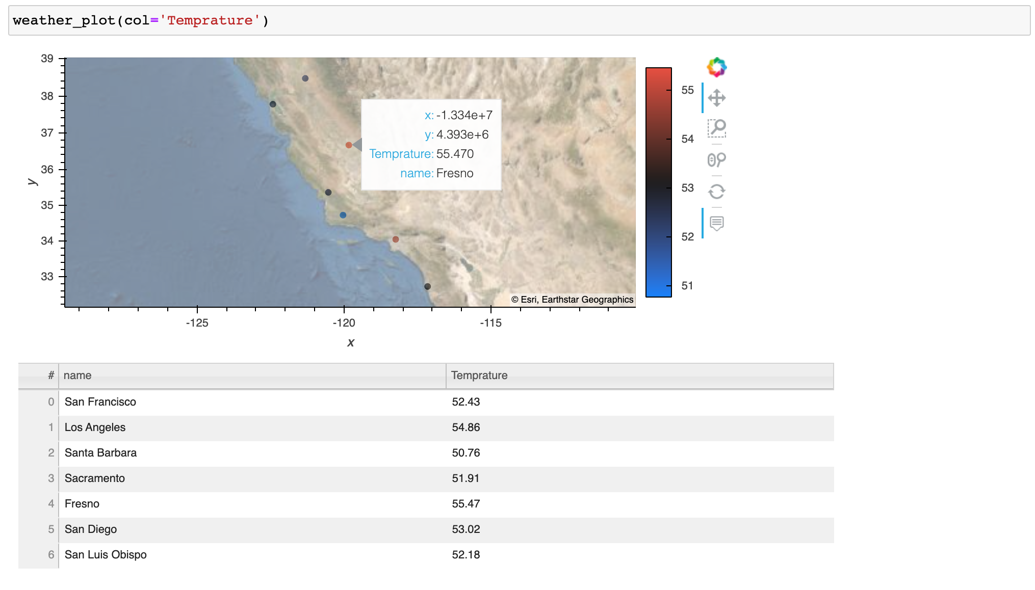
먼저 간단한 함수를 만들어 보겠습니다weather_plot도시 이름이 지정된지도에 날씨 데이터를 플로팅하고 플롯과 데이터를 모두 반환합니다.
플로팅 기능이 준비되면 새로 고칠 수있는 대시 보드를 만들 수 있습니다.나는param.Action버튼을 클릭 할 때마다 업데이트를 트리거하는 함수새롭게 하다.또한param.ObjectSelector플로팅에 관심이있는 데이터 프레임 열의 드롭 다운 메뉴를 생성하고param.ObjectSelector드롭 다운 메뉴에서 다른 옵션을 선택할 때마다 업데이트를 트리거합니다.그런 다음@ param.depends ( 'action', 'select_column')데코레이터는get_plot클릭 할 때마다 다시 실행되는 기능새롭게 하다버튼을 누르거나 다른 열을 선택하십시오.
Data scientists use data visualization to communicate data and generate insights. It’s essential for data scientists to know how to create meaningful visualization dashboards, especially real-time dashboards. This article talks about two ways to get your real-time dashboard in Python:
First, we use streaming data and create an auto-updated streaming dashboard.
Second, we use a “Refresh” button to refresh the dashboard whenever we need the dashboard to be refreshed.
For demonstration purposes, the plots and dashboards are very basic, but you will get the idea of how we do a real-time dashboard.
To show howwe create this dashboard with a real-world API, we use weather data from the OpenWeather API as an example in this article.
If you would like to try out the code mentioned in this article, you will need to get access to the OpenWeather weather API. You can sign up at the Open Weather website and then get the API keys.
Set up
Before going into the code, let’s install the needed packages. I have created an enviornment.yml file. Please download this file and run the following to create and activate the environment.
Alternatively, if you want to install all the packages on your own, please conda install datashader holoviews hvplot notebook numpy pandas panel param requests streamz. If you see any issues, the Python version and package versions I am using are noted in the environment.yml.
Import packages
Here we import the packages used for this article:
Streaming data and dashboard
First, we make a function weather_data to get weather data for a list of cities using the OpenWeather API. The output is a pandas dataframe with each row representing each city.
Second, we use streamzto create a streaming dataframe based on San Francisco’s weather data. The function streaming_weather_data is used as a callback function by the PeriodicDataFrame function to create a streamzstreaming dataframe df. streamzdocs documented how PeriodicDataFrame works:
streamz provides a high-level convenience class for this purpose, called a PeriodicDataFrame. A PeriodicDataFrame uses Python’s asyncio event loop (used as part of Tornado in Jupyter and other interactive frameworks) to call a user-provided function at a regular interval, collecting the results and making them available for later processing.
The streamzstreaming dataframe df looks like this, with values updated every 30s (since we set interval=’30').
Third, we make some very basic plots using hvPlot to plot the streamzdataframe, and then we use panel to organize the plots and put everything in a dashboard. If you would like to know more about how to usehvPlot to plot streamzdataframe, please see hvPlot docs.
Here is what the dashboard looks like. Since the streaming dataframe updates every 30s, this dashboard will automatically update every 30s as well. Here we see that Temperature changed, while humidity and wind speed did not.
Great, now you know how to make a streaming dataframe and a streaming dashboard.
If you would like to learn more, here is a great video tutorial on the streaming dashboard by my friend Dr. Jim Bednar. Please check it out!
Refresh dashboard
Sometimes, we don’t really need a streaming dashboard. Instead, we might just like to refresh the dashboard whenever we see it. In this section, I am going to show you how to make a “Refresh” button in your dashboard and refresh the dashboard with new data whenever you click “Refresh”.
First, let’s make a simple function weather_plot to plot weather data on a map given city names and return both the plot and the data.
With the plotting function ready, we can start making the refreshable dashboard. I use the param.Action function to trigger an update whenever we click on the button Refresh. In addition, I use the param.ObjectSelector function to create a dropdown menu of the dataframe columns we are interested in plotting and param.ObjectSelector trigger an update whenever we select a different option in the dropdown menu. Then the @param.depends('action', 'select_column') decorator tells the get_plot function to rerun whenever we click the Refresh button or select another column.
Here is what the refresh dashboard looks like:
Finally, we can use panel to combine the two dashboards we created.
Deployment
Our final dashboard pane is a panel object, which can be served by running:
panel serve realtime_dashboard.py
or
panel serve realtime_dashboard.ipynb
For more information on panel deployment, please refer to the paneldocs.
Now you know how to make a real-time streaming dashboard and a refreshable dashboard in python using hvplot , paneland streamz. Hope you find this article helpful!