
2021년 3월 2일 모바일 게임 매출 순위
| Rank | Game | Publisher |
|---|---|---|
| 1 | 리니지M | NCSOFT |
| 2 | 리니지2M | NCSOFT |
| 3 | 그랑사가 | NPIXEL |
| 4 | 기적의 검 | 4399 KOREA |
| 5 | Cookie Run: Kingdom – Kingdom Builder & Battle RPG | Devsisters Corporation |
| 6 | 세븐나이츠2 | Netmarble |
| 7 | V4 | NEXON Company |
| 8 | Genshin Impact | miHoYo Limited |
| 9 | 바람의나라: 연 | NEXON Company |
| 10 | 블레이드&소울 레볼루션 | Netmarble |
| 11 | 리니지2 레볼루션 | Netmarble |
| 12 | 뮤 아크엔젤 | Webzen Inc. |
| 13 | 라이즈 오브 킹덤즈 | LilithGames |
| 14 | KartRider Rush+ | NEXON Company |
| 15 | R2M | Webzen Inc. |
| 16 | S.O.S:스테이트 오브 서바이벌 | KingsGroup Holdings |
| 17 | A3: 스틸얼라이브 | Netmarble |
| 18 | FIFA ONLINE 4 M by EA SPORTS™ | NEXON Company |
| 19 | Pmang Poker : Casino Royal | NEOWIZ corp |
| 20 | Roblox | Roblox Corporation |
| 21 | Summoners War | Com2uS |
| 22 | Brawl Stars | Supercell |
| 23 | 가디언 테일즈 | Kakao Games Corp. |
| 24 | 삼국지 전략판 | Qookka Games |
| 25 | 미르4 | Wemade Co., Ltd |
| 26 | 에오스 레드 | BluePotion Games |
| 27 | 카운터사이드 | NEXON Company |
| 28 | 검은강호2: 이터널 소울 | 9SplayDeveloper |
| 29 | Cookie Run: OvenBreak – Endless Running Platformer | Devsisters Corporation |
| 30 | 검은사막 모바일 | PEARL ABYSS |
| 31 | 찐삼국 | ICEBIRD GAMES |
| 32 | Epic Seven | Smilegate Megaport |
| 33 | 라그나로크 오리진 | GRAVITY Co., Ltd. |
| 34 | 메이플스토리M | NEXON Company |
| 35 | Lords Mobile: Kingdom Wars | IGG.COM |
| 36 | 한게임 포커 | NHN BIGFOOT |
| 37 | Age of Z Origins | Camel Games Limited |
| 38 | PUBG MOBILE | KRAFTON, Inc. |
| 39 | Gardenscapes | Playrix |
| 40 | Top War: Battle Game | Topwar Studio |
| 41 | AFK 아레나 | LilithGames |
| 42 | 어비스(ABYSS) | StairGames Inc. |
| 43 | Empires & Puzzles: Epic Match 3 | Small Giant Games |
| 44 | 슬램덩크 | DeNA HONG KONG LIMITED |
| 45 | Homescapes | Playrix |
| 46 | 그랑삼국 | YOUZU(SINGAPORE)PTE.LTD. |
| 47 | 갑부: 장사의 시대 | BLANCOZONE NETWORK KOREA |
| 48 | 라그나로크M: TRINITY | GRAVITY Co., Ltd. |
| 49 | 컴투스프로야구2021 | Com2uS |
| 50 | FIFA Mobile | NEXON Company |
2021년 3월 1일 모바일 게임 매출 순위
| Rank | Game | Publisher |
|---|---|---|
| 1 | 리니지M | NCSOFT |
| 2 | 리니지2M | NCSOFT |
| 3 | 그랑사가 | NPIXEL |
| 4 | Cookie Run: Kingdom – Kingdom Builder & Battle RPG | Devsisters Corporation |
| 5 | 기적의 검 | 4399 KOREA |
| 6 | 세븐나이츠2 | Netmarble |
| 7 | V4 | NEXON Company |
| 8 | Genshin Impact | miHoYo Limited |
| 9 | 라이즈 오브 킹덤즈 | LilithGames |
| 10 | KartRider Rush+ | NEXON Company |
| 11 | 뮤 아크엔젤 | Webzen Inc. |
| 12 | 블레이드&소울 레볼루션 | Netmarble |
| 13 | 바람의나라: 연 | NEXON Company |
| 14 | 리니지2 레볼루션 | Netmarble |
| 15 | S.O.S:스테이트 오브 서바이벌 | KingsGroup Holdings |
| 16 | R2M | Webzen Inc. |
| 17 | Roblox | Roblox Corporation |
| 18 | 가디언 테일즈 | Kakao Games Corp. |
| 19 | 삼국지 전략판 | Qookka Games |
| 20 | Brawl Stars | Supercell |
| 21 | 미르4 | Wemade Co., Ltd |
| 22 | Summoners War | Com2uS |
| 23 | A3: 스틸얼라이브 | Netmarble |
| 24 | Cookie Run: OvenBreak – Endless Running Platformer | Devsisters Corporation |
| 25 | 카운터사이드 | NEXON Company |
| 26 | 찐삼국 | ICEBIRD GAMES |
| 27 | FIFA ONLINE 4 M by EA SPORTS™ | NEXON Company |
| 28 | 검은강호2: 이터널 소울 | 9SplayDeveloper |
| 29 | 에오스 레드 | BluePotion Games |
| 30 | 검은사막 모바일 | PEARL ABYSS |
| 31 | Lords Mobile: Kingdom Wars | IGG.COM |
| 32 | Epic Seven | Smilegate Megaport |
| 33 | PUBG MOBILE | KRAFTON, Inc. |
| 34 | Top War: Battle Game | Topwar Studio |
| 35 | 라그나로크 오리진 | GRAVITY Co., Ltd. |
| 36 | Age of Z Origins | Camel Games Limited |
| 37 | Gardenscapes | Playrix |
| 38 | 메이플스토리M | NEXON Company |
| 39 | Empires & Puzzles: Epic Match 3 | Small Giant Games |
| 40 | 어비스(ABYSS) | StairGames Inc. |
| 41 | 슬램덩크 | DeNA HONG KONG LIMITED |
| 42 | 그랑삼국 | YOUZU(SINGAPORE)PTE.LTD. |
| 43 | Pmang Poker : Casino Royal | NEOWIZ corp |
| 44 | AFK 아레나 | LilithGames |
| 45 | Homescapes | Playrix |
| 46 | 한게임 포커 | NHN BIGFOOT |
| 47 | 라그나로크M: TRINITY | GRAVITY Co., Ltd. |
| 48 | 갑부: 장사의 시대 | BLANCOZONE NETWORK KOREA |
| 49 | 컴투스프로야구2021 | Com2uS |
| 50 | Pokémon GO | Niantic, Inc. |
Pandas May Not Be the King of the Jungle After All -번역
판다는 결국 정글의 왕이 아닐 수도있다
약간 편향된 비교

Pandas는 표 형식의 중소 규모 데이터로 데이터 분석 및 조작 작업을 지배하고 있습니다.데이터 과학 생태계에서 가장 인기있는 라이브러리입니다.
저는 Pandas의 열렬한 팬이며 데이터 과학 여정을 시작한 이래로 Pandas를 사용해 왔습니다.나는 지금까지 그것을 좋아하지만 Pandas에 대한 나의 열정은 내가 다른 도구를 시도하는 것을 방해하지 않아야합니다.
나는 다른 것을 비교하는 것을 좋아한다 도구 및 라이브러리.내 비교 방법은 둘 다에 대해 동일한 작업을 수행하는 것입니다.나는 보통 내가 이미 알고있는 것을 내가 배우고 싶은 새로운 것과 비교한다.새로운 도구를 배우게 할뿐만 아니라 이미 알고있는 것을 연습하는데도 도움이됩니다.
제 동료 중 한 명이 저에게 R 용 “data.table”패키지를 사용해 보라고했습니다. 그는 데이터 분석 및 조작 작업에 대해 Pandas보다 더 효율적이라고 주장했습니다.그래서 나는 그것을 시도했습니다.”data.table”을 사용하여 특정 작업을 수행하는 것이 얼마나 간단한 지 감명을 받았습니다.
이 기사에서는 Pandas와 data.table을 비교하기 위해 몇 가지 예를 살펴 보겠습니다.데이터 분석 라이브러리의 기본 선택을 Pandas에서 data.table로 변경해야하는지 여전히 논쟁 중입니다.그러나 data.table이 Pandas를 대체하는 첫 번째 후보라고 말할 수 있습니다.
더 이상 고민하지 않고 예제부터 시작하겠습니다.멜버른 주택의 작은 샘플을 사용합니다.데이터 세트예제는 Kaggle에서 사용할 수 있습니다.
첫 번째 단계는 각각 Pandas 및 data.table에 대한 read_csv 및 fread 함수에 의해 수행되는 데이터 세트를 읽는 것입니다.구문은 거의 동일합니다.
# 팬더
numpy를 np로 가져 오기
팬더를 pd로 가져 오기melbourne = pd.read_csv ( "/ content / melb_data.csv",
usecols = [ 'Price', 'Landsize', 'Distance', 'Type', 'Regionname'])# data.table
라이브러리 (data.table)melb & lt;-fread ( "~ / Downloads / melb_data.csv", select = c ( 'Price', 'Landsize', 'Distance', 'Type', 'Regionname'))
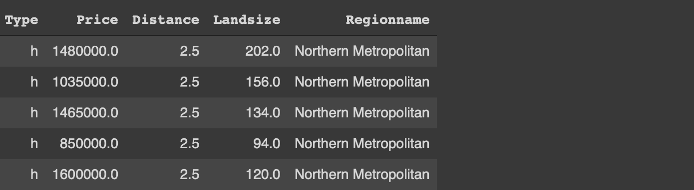
두 라이브러리 모두 열 값을 기반으로 행을 필터링하는 간단한 방법을 제공합니다.유형이 “h”이고 거리가 4보다 큰 행을 필터링하려고합니다.
# 팬더melb [(melb.Type == 'h') & amp;(melb. 거리> 4)]# data.tablemelb [유형 == 'h'& amp;거리 & gt;4]
우리는 data.table에만 열 이름을 쓰는 반면 Pandas는 데이터 프레임의 이름도 필요로합니다.
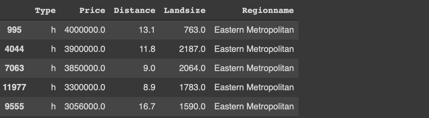
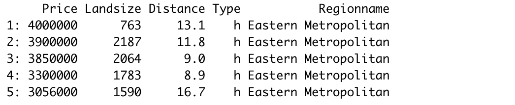
다음 작업은 데이터 포인트 (즉, 행)를 정렬하는 것입니다.지역 이름을 기준으로 오름차순으로 정렬 한 다음 가격을 기준으로 내림차순으로 정렬해야합니다.
두 라이브러리를 사용하여이 작업을 수행하는 방법은 다음과 같습니다.
# 팬더melb.sort_values (by = [ 'Regionname', 'Price'], ascending = [True, False])# data.tablemelb [주문 (지역 명,-가격)]
논리는 동일합니다.열과 순서 (오름차순 또는 내림차순)가 지정됩니다.그러나 구문은 data.table을 사용하면 훨씬 간단합니다.
data.table의 또 다른 장점은 Pandas의 경우가 아닌 정렬 후 인덱스가 재설정된다는 것입니다.색인을 재설정하려면 추가 매개 변수 (ignore_index)를 사용해야합니다.
데이터 분석의 또 다른 일반적인 작업은 열의 범주를 기반으로 관찰 (즉, 행)을 그룹화하는 것입니다.그런 다음 각 그룹의 숫자 열에 대한 통계를 계산합니다.
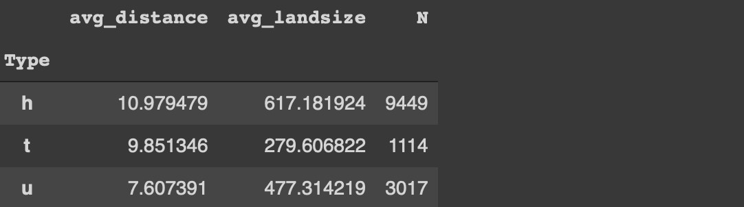
유형 열의 각 범주에 대한 주택의 평균 가격과 토지 크기를 계산해 보겠습니다.또한 각 범주의 주택 수를 확인하려고합니다.
# 팬더melb [[ '시간', '먼', '토지 크기']] \
.groupby ( 'Type'). agg ([ 'mean', 'count'])
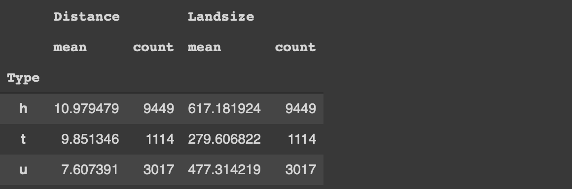
Pandas에서는 관심있는 열을 선택하고 groupby 함수를 사용합니다.그런 다음 집계 함수가 지정됩니다.
편집 : 감사합니다헨릭 보 라르센머리 위로.나는 agg 기능의 유연성을 간과했습니다.열을 먼저 선택하지 않고도 동일한 작업을 수행 할 수 있습니다.
# 팬더melb.groupby ( '유형') .agg (
avg_distance = ( '거리', '평균'),
avg_landsize = ( 'Landsize', 'mean'),
N = ( '거리', '개수')
)
다음은 data.table로 동일한 작업을 수행하는 방법입니다.
# data.tablemelb [,. (mean (거리), mean (Landsize), .N), by = 'Type']
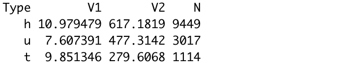
“by”매개 변수를 사용하여 그룹화에 사용할 열을 선택합니다.열을 선택하는 동안 집계 함수가 지정됩니다.판다보다 간단합니다.
또한 필터링 구성 요소를 추가하고 비용이 1 백만 미만인 주택에 대해 동일한 통계를 계산해 보겠습니다.
# 팬더melb [melb. 가격 & lt;1000000] [[ '유형', '거리', '토지 크기']] \
.groupby ( 'Type'). agg ([ 'mean', 'count'])# data.tablemelb [가격 & lt;1000000,. (mean (거리), mean (Landsize), .N), by = 'Type']
필터링 구성 요소는 data.table과 동일한 대괄호로 지정됩니다.반면에 Pandas의 다른 모든 작업보다 먼저 필터링을 수행해야합니다.
결론
이 기사에서 다루는 내용은 일반적인 데이터 분석 프로세스에서 수행되는 일반적인 작업입니다.물론이 두 라이브러리가 제공하는 더 많은 기능이 있습니다.따라서이 기사는 포괄적 인 비교가 아닙니다.그러나 두 가지 모두에서 작업을 처리하는 방법에 대한 일부 정보를 제공합니다.
특정 작업을 완료하기위한 구문과 접근 방식에만 집중했습니다.메모리 및 속도와 같은 성능 관련 문제는 아직 발견되지 않았습니다.
요약하면 data.table은 나를 위해 Pandas를 대체 할 수있는 강력한 후보라고 생각합니다.또한 자주 사용하는 다른 라이브러리에 따라 다릅니다.Python 라이브러리를 많이 사용하는 경우 Pandas를 고수하는 것이 좋습니다.그러나 data.table은 확실히 시도해 볼 가치가 있습니다.
읽어 주셔서 감사합니다.의견이 있으면 알려주세요.
Pandas May Not Be the King of the Jungle After All
Pandas May Not Be the King of the Jungle After All
A slightly biased comparison
Pandas is dominating the data analysis and manipulation tasks with small-to-medium sized data in tabular form. It is arguably the most popular library in the data science ecosystem.
I’m a big fan of Pandas and have been using it since I started my data science journey. I love it so far but my passion for Pandas should not and does not prevent me from trying different tools.
I like to try comparing different tools and libraries. My way of comparison is to do the same tasks with both. I usually compare what I already know with the new one I want to learn. It not only makes me learn a new tool but also helps me practice what I already know.
One of my colleagues told me to try the “data.table” package for R. He argued that it is more efficient than Pandas for data analysis and manipulation tasks. So I gave it a try. I was impressed by how simple it was to accomplish certain tasks with “data.table”.
In this article, I will go over several examples to make a comparison between Pandas and data.table. I’m still debating if I should change my default choice of data analysis library from Pandas to data.table. However, I can say that data.table is the first candidate to replace Pandas.
Without further ado, let’s start with the examples. We will use a small sample from the Melbourne housing dataset available on Kaggle for the examples.
The first step is to read the dataset which is done by the read_csv and fread functions for Pandas and data.table, respectively. The syntax is almost the same.
#Pandas
import numpy as np
import pandas as pdmelb = pd.read_csv("/content/melb_data.csv",
usecols = ['Price','Landsize','Distance','Type', 'Regionname'])#data.table
library(data.table)melb <- fread("~/Downloads/melb_data.csv", select=c('Price','Landsize','Distance','Type', 'Regionname'))
Both libraries provide simple ways of filtering rows based on column values. We want to filter the rows with type “h” and distance greater than 4.
#Pandasmelb[(melb.Type == 'h') & (melb.Distance > 4)]#data.tablemelb[Type == 'h' & Distance > 4]
We only write the column names in data.table whereas Pandas requires to with the name of the dataframe as well.
The next task is to sort the data points (i.e. rows). Consider we need to sort the rows by region name in ascending order and then by price in descending order.
Here is how we can accomplish this task with both libraries.
#Pandasmelb.sort_values(by=['Regionname','Price'], ascending=[True, False])#data.tablemelb[order(Regionname, -Price)]
The logic is the same. The columns and the order (ascending or descending) are specified. However, the syntax is much simple with data.table.
Another advantage of data.table is that the indices are reset after sorting which is not the case with Pandas. We need to use an additional parameter (ignore_index) to reset the index.
Another common task in data analysis is to group observations (i.e. rows) based on the categories in a column. We then calculate statistics on numerical columns for each group.
Let’s calculate the average price and land size of the houses for each category in the type column. We also want to see the number of houses in each category.
#Pandasmelb[['Type','Distance','Landsize']]\
.groupby('Type').agg(['mean','count'])
With Pandas, we select the columns of interest and use the groupby function. Then the aggregations functions are specified.
Edit: Thanks Henrik Bo Larsen for the heads up. I overlooked the flexibility of the agg function. We can do the same operation without selecting the columns first:
#Pandasmelb.groupby('Type').agg(
   avg_distance = ('Distance', 'mean'),
   avg_landsize = ('Landsize', 'mean'),
   N = ('Distance', 'count')
)
Here is how we do the same tasks with data.table:
#data.tablemelb[, .(mean(Distance), mean(Landsize), .N), by='Type']
We use the “by” parameter to select the column to be used in grouping. The aggregate functions are specified while selecting the columns. It is simpler than Pandas.
Let’s also add a filtering component and calculate the same statistics for houses that cost less than 1 million.
#Pandasmelb[melb.Price < 1000000][['Type','Distance','Landsize']]\
.groupby('Type').agg(['mean','count'])#data.tablemelb[Price < 1000000, .(mean(Distance), mean(Landsize), .N), by='Type']
The filtering component is specified in the same square brackets with data.table. On the other hand, we need to do the filtering before all other operations in Pandas.
Conclusion
What we covered in this article are common tasks done in a typical data analysis process. There are, of course, many more functions these two libraries provide. Thus, this article is not a comprehensive comparison. However, it sheds some light on how tasks are handled in both.
I have only focused on the syntax and the approach to complete certain operations. Performance related issues such as memory and speed are yet to discover.
To sum up, I feel like data.table is a strong candidate to replace Pandas for me. It also depends on the other libraries you frequently use. If you heavily use Python libraries, you may want to stick with Pandas. However, data.table is definitely worth a try.
Thank you for reading. Please let me know if you have any feedback.