
Pandas May Not Be the King of the Jungle After All
A slightly biased comparison

Pandas is dominating the data analysis and manipulation tasks with small-to-medium sized data in tabular form. It is arguably the most popular library in the data science ecosystem.
I’m a big fan of Pandas and have been using it since I started my data science journey. I love it so far but my passion for Pandas should not and does not prevent me from trying different tools.
I like to try comparing different tools and libraries. My way of comparison is to do the same tasks with both. I usually compare what I already know with the new one I want to learn. It not only makes me learn a new tool but also helps me practice what I already know.
One of my colleagues told me to try the “data.table” package for R. He argued that it is more efficient than Pandas for data analysis and manipulation tasks. So I gave it a try. I was impressed by how simple it was to accomplish certain tasks with “data.table”.
In this article, I will go over several examples to make a comparison between Pandas and data.table. I’m still debating if I should change my default choice of data analysis library from Pandas to data.table. However, I can say that data.table is the first candidate to replace Pandas.
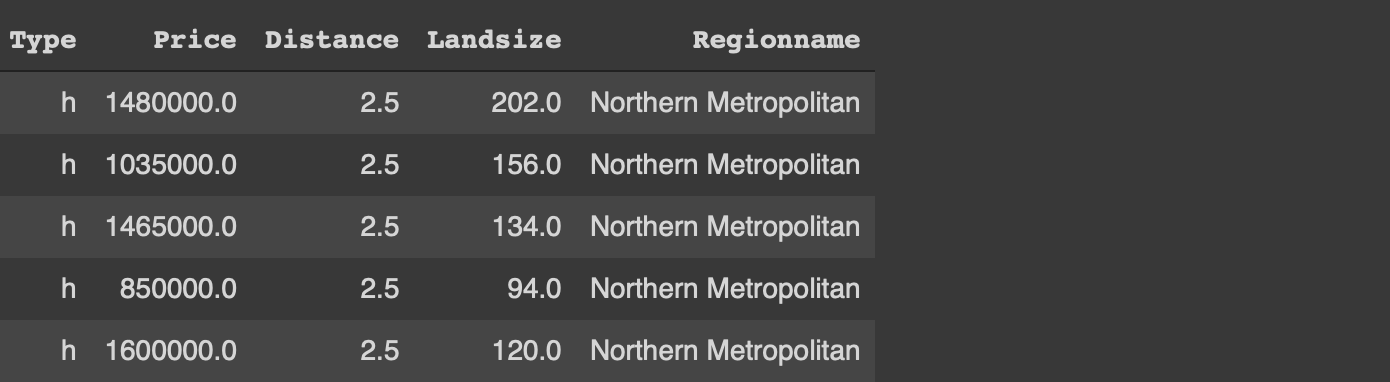
Without further ado, let’s start with the examples. We will use a small sample from the Melbourne housing dataset available on Kaggle for the examples.
The first step is to read the dataset which is done by the read_csv and fread functions for Pandas and data.table, respectively. The syntax is almost the same.
#Pandas
import numpy as np
import pandas as pdmelb = pd.read_csv("/content/melb_data.csv",
usecols = ['Price','Landsize','Distance','Type', 'Regionname'])#data.table
library(data.table)melb <- fread("~/Downloads/melb_data.csv", select=c('Price','Landsize','Distance','Type', 'Regionname'))
Both libraries provide simple ways of filtering rows based on column values. We want to filter the rows with type “h” and distance greater than 4.
#Pandasmelb[(melb.Type == 'h') & (melb.Distance > 4)]#data.tablemelb[Type == 'h' & Distance > 4]
We only write the column names in data.table whereas Pandas requires to with the name of the dataframe as well.
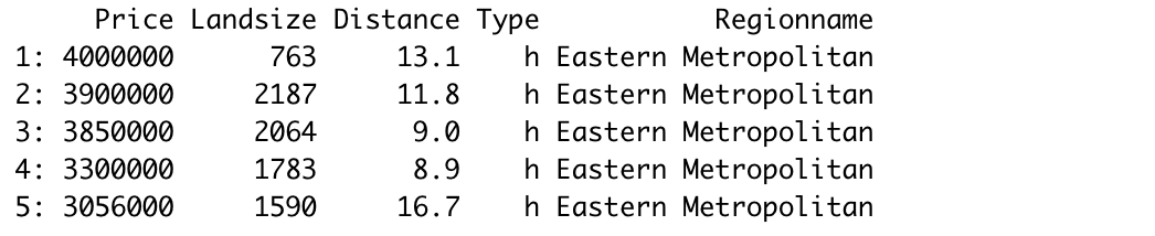
The next task is to sort the data points (i.e. rows). Consider we need to sort the rows by region name in ascending order and then by price in descending order.
Here is how we can accomplish this task with both libraries.
#Pandasmelb.sort_values(by=['Regionname','Price'], ascending=[True, False])#data.tablemelb[order(Regionname, -Price)]
The logic is the same. The columns and the order (ascending or descending) are specified. However, the syntax is much simple with data.table.
Another advantage of data.table is that the indices are reset after sorting which is not the case with Pandas. We need to use an additional parameter (ignore_index) to reset the index.

Another common task in data analysis is to group observations (i.e. rows) based on the categories in a column. We then calculate statistics on numerical columns for each group.
Let’s calculate the average price and land size of the houses for each category in the type column. We also want to see the number of houses in each category.
#Pandasmelb[['Type','Distance','Landsize']]\
.groupby('Type').agg(['mean','count'])
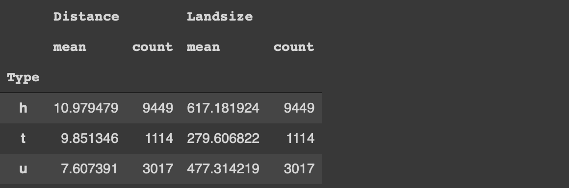
With Pandas, we select the columns of interest and use the groupby function. Then the aggregations functions are specified.
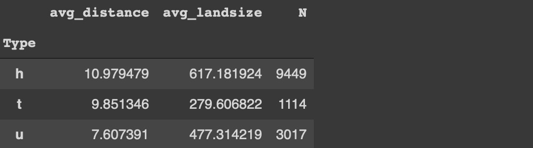
Edit: Thanks Henrik Bo Larsen for the heads up. I overlooked the flexibility of the agg function. We can do the same operation without selecting the columns first:
#Pandasmelb.groupby('Type').agg(
   avg_distance = ('Distance', 'mean'),
   avg_landsize = ('Landsize', 'mean'),
   N = ('Distance', 'count')
)
Here is how we do the same tasks with data.table:
#data.tablemelb[, .(mean(Distance), mean(Landsize), .N), by='Type']
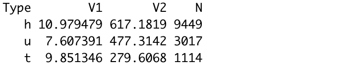
We use the “by” parameter to select the column to be used in grouping. The aggregate functions are specified while selecting the columns. It is simpler than Pandas.
Let’s also add a filtering component and calculate the same statistics for houses that cost less than 1 million.
#Pandasmelb[melb.Price < 1000000][['Type','Distance','Landsize']]\
.groupby('Type').agg(['mean','count'])#data.tablemelb[Price < 1000000, .(mean(Distance), mean(Landsize), .N), by='Type']
The filtering component is specified in the same square brackets with data.table. On the other hand, we need to do the filtering before all other operations in Pandas.
Conclusion
What we covered in this article are common tasks done in a typical data analysis process. There are, of course, many more functions these two libraries provide. Thus, this article is not a comprehensive comparison. However, it sheds some light on how tasks are handled in both.
I have only focused on the syntax and the approach to complete certain operations. Performance related issues such as memory and speed are yet to discover.
To sum up, I feel like data.table is a strong candidate to replace Pandas for me. It also depends on the other libraries you frequently use. If you heavily use Python libraries, you may want to stick with Pandas. However, data.table is definitely worth a try.
Thank you for reading. Please let me know if you have any feedback.